Assessing Model Fit C OR R E L ATION AN D R E G R E SSION IN R - PowerPoint PPT Presentation
Assessing Model Fit C OR R E L ATION AN D R E G R E SSION IN R Ben Ba u mer Assistant Professor at Smith College Ho w w ell does o u r te x tbook model fit ? ggplot(data = textbooks, aes(x = amazNew, y = uclaNew)) + geom_point() +
Assessing Model Fit C OR R E L ATION AN D R E G R E SSION IN R Ben Ba u mer Assistant Professor at Smith College
Ho w w ell does o u r te x tbook model fit ? ggplot(data = textbooks, aes(x = amazNew, y = uclaNew)) + geom_point() + geom_smooth(method = "lm", se = FALSE) CORRELATION AND REGRESSION IN R
Ho w w ell does o u r poss u m model fit ? ggplot(data = possum, aes(y = totalL, x = tailL)) + geom_point() + geom_smooth(method = "lm", se = FALSE) CORRELATION AND REGRESSION IN R
S u ms of sq u ared de v iations CORRELATION AND REGRESSION IN R
SSE library(broom) mod_possum <- lm(totalL ~ tailL, data = possum) mod_possum %>% augment() %>% summarize(SSE = sum(.resid^2), SSE_also = (n() - 1) * var(.resid)) SSE SSE_also 1 1301 1301 CORRELATION AND REGRESSION IN R
RMSE CORRELATION AND REGRESSION IN R
Resid u al standard error ( poss u ms ) summary(mod_possum) Call: lm(formula = totalL ~ tailL, data = possum) Residuals: Min 1Q Median 3Q Max -9.210 -2.326 0.179 2.777 6.790 Coefficients: Estimate Std. Error t value Pr(>|t|) (Intercept) 41.04 6.66 6.16 1.4e-08 tailL 1.24 0.18 6.93 3.9e-10 Residual standard error: 3.57 on 102 degrees of freedom Multiple R-squared: 0.32, Adjusted R-squared: 0.313 F-statistic: 48 on 1 and 102 DF, p-value: 3.94e-10 CORRELATION AND REGRESSION IN R
Resid u al standard error ( te x tbooks ) lm(uclaNew ~ amazNew, data = textbooks) %>% summary() Call: lm(formula = uclaNew ~ amazNew, data = textbooks) Residuals: Min 1Q Median 3Q Max -34.78 -4.57 0.58 4.01 39.00 Coefficients: Estimate Std. Error t value Pr(>|t|) (Intercept) 0.9290 1.9354 0.48 0.63 amazNew 1.1990 0.0252 47.60 <2e-16 Residual standard error: 10.5 on 71 degrees of freedom Multiple R-squared: 0.97, Adjusted R-squared: 0.969 F-statistic: 2.27e+03 on 1 and 71 DF, p-value: <2e-16 CORRELATION AND REGRESSION IN R
Let ' s practice ! C OR R E L ATION AN D R E G R E SSION IN R
Comparing model fits C OR R E L ATION AN D R E G R E SSION IN R Ben Ba u mer Assistant Professor at Smith College
Ho w w ell does o u r te x tbook model fit ? ggplot(data = textbooks, aes(x = amazNew, y = uclaNew)) + geom_point() + geom_smooth(method = "lm", se = FALSE) CORRELATION AND REGRESSION IN R
Ho w w ell does o u r poss u m model fit ? ggplot(data = possum, aes(y = totalL, x = tailL)) + geom_point() + geom_smooth(method = "lm", se = FALSE) CORRELATION AND REGRESSION IN R
N u ll ( a v erage ) model For all obser v ations … CORRELATION AND REGRESSION IN R
Vis u ali z ation of n u ll model CORRELATION AND REGRESSION IN R
SSE , n u ll model mod_null <- lm(totalL ~ 1, data = possum) mod_null %>% augment(possum) %>% summarize(SSE = sum(.resid^2)) SSE 1 1914 CORRELATION AND REGRESSION IN R
SSE , o u r model mod_possum <- lm(totalL ~ tailL, data = possum) mod_possum %>% augment() %>% summarize(SSE = sum(.resid^2)) SSE 1 1301 CORRELATION AND REGRESSION IN R
Coefficient of determination SST is the SSE for the n u ll model CORRELATION AND REGRESSION IN R
Connection to correlation For simple linear regression ... CORRELATION AND REGRESSION IN R
S u mmar y summary(mod_possum) Call: lm(formula = totalL ~ tailL, data = possum) Residuals: Min 1Q Median 3Q Max -9.210 -2.326 0.179 2.777 6.790 Coefficients: Estimate Std. Error t value Pr(>|t|) (Intercept) 41.04 6.66 6.16 1.4e-08 tailL 1.24 0.18 6.93 3.9e-10 Residual standard error: 3.57 on 102 degrees of freedom Multiple R-squared: 0.32, Adjusted R-squared: 0.313 F-statistic: 48 on 1 and 102 DF, p-value: 3.94e-10 CORRELATION AND REGRESSION IN R
O v er - reliance on R - sq u ared CORRELATION AND REGRESSION IN R
Let ' s practice ! C OR R E L ATION AN D R E G R E SSION IN R
Un u s u al Points C OR R E L ATION AN D R E G R E SSION IN R Ben Ba u mer Assistant Professor at Smith College
Un u s u al points regulars <- mlbBat10 %>% filter(AB > 400) ggplot(data = regulars, aes(x = SB, y = HR)) + geom_point() + geom_smooth(method = "lm", se = 0) CORRELATION AND REGRESSION IN R
Un u s u al points regulars <- mlbBat10 %>% filter(AB > 400) ggplot(data = regulars, aes(x = SB, y = HR)) + geom_point() + geom_smooth(method = "lm", se = 0) CORRELATION AND REGRESSION IN R
Un u s u al points regulars <- mlbBat10 %>% filter(AB > 400) ggplot(data = regulars, aes(x = SB, y = HR)) + geom_point() + geom_smooth(method = "lm", se = 0) CORRELATION AND REGRESSION IN R
Un u s u al points regulars <- mlbBat10 %>% filter(AB > 400) ggplot(data = regulars, aes(x = SB, y = HR)) + geom_point() + geom_smooth(method = "lm", se = 0) CORRELATION AND REGRESSION IN R
Le v erage CORRELATION AND REGRESSION IN R
Le v erage comp u tations library(broom) mod <- lm(HR ~ SB, data = regulars) mod %>% augment() %>% arrange(desc(.hat)) %>% select(HR, SB, .fitted, .resid, .hat) %>% head() HR SB .fitted .resid .hat 1 1 68 2.383 -1.383 0.13082 2 2 52 6.461 -4.461 0.07034 3 5 50 6.971 -1.971 0.06417 4 19 47 7.736 11.264 0.05550 5 5 47 7.736 -2.736 0.05550 6 1 42 9.010 -8.010 0.04261 CORRELATION AND REGRESSION IN R
Le v erage comp u tations library(broom) mod <- lm(HR ~ SB, data = regulars) mod %>% augment() %>% arrange(desc(.hat)) %>% select(HR, SB, .fitted, .resid, .hat) %>% head() HR SB .fitted .resid .hat 1 1 68 2.383 -1.383 0.13082 # Juan Pierre 2 2 52 6.461 -4.461 0.07034 3 5 50 6.971 -1.971 0.06417 4 19 47 7.736 11.264 0.05550 5 5 47 7.736 -2.736 0.05550 6 1 42 9.010 -8.010 0.04261 CORRELATION AND REGRESSION IN R
Consider Ricke y Henderson … CORRELATION AND REGRESSION IN R
Consider Ricke y Henderson … CORRELATION AND REGRESSION IN R
Consider Ricke y Henderson … CORRELATION AND REGRESSION IN R
Infl u ence v ia Cook ' s distance mod <- lm(HR ~ SB, data = regulars_plus) mod %>% augment() %>% arrange(desc(.cooksd)) %>% select(HR, SB, .fitted, .resid, .hat, .cooksd) %>% head() HR SB .fitted .resid .hat .cooksd 1 28 65 5.770 22.230 0.105519 0.33430 2 54 9 17.451 36.549 0.006070 0.04210 3 34 26 13.905 20.095 0.013150 0.02797 4 19 47 9.525 9.475 0.049711 0.02535 5 39 0 19.328 19.672 0.010479 0.02124 6 42 14 16.408 25.592 0.006061 0.02061 CORRELATION AND REGRESSION IN R
Infl u ence v ia Cook ' s distance mod <- lm(HR ~ SB, data = regulars_plus) mod %>% augment() %>% arrange(desc(.cooksd)) %>% select(HR, SB, .fitted, .resid, .hat, .cooksd) %>% head() HR SB .fitted .resid .hat .cooksd 1 28 65 5.770 22.230 0.105519 0.33430 # Henderson 2 54 9 17.451 36.549 0.006070 0.04210 3 34 26 13.905 20.095 0.013150 0.02797 4 19 47 9.525 9.475 0.049711 0.02535 5 39 0 19.328 19.672 0.010479 0.02124 6 42 14 16.408 25.592 0.006061 0.02061 CORRELATION AND REGRESSION IN R
Let ' s practice ! C OR R E L ATION AN D R E G R E SSION IN R
Dealing w ith O u tliers C OR R E L ATION AN D R E G R E SSION IN R Ben Ba u mer Assistant Professor at Smith College
Dealing w ith o u tliers ggplot(data = regulars_plus, aes(x = SB, y = HR)) + geom_point() + geom_smooth(method = "lm", se = 0) CORRELATION AND REGRESSION IN R
Dealing w ith o u tliers ggplot(data = regulars_plus, aes(x = SB, y = HR)) + geom_point() + geom_smooth(method = "lm", se = 0) CORRELATION AND REGRESSION IN R
Dealing w ith o u tliers ggplot(data = regulars_plus, aes(x = SB, y = HR)) + geom_point() + geom_smooth(method = "lm", se = 0) CORRELATION AND REGRESSION IN R
The f u ll model coef(lm(HR ~ SB, data = regulars_plus)) (Intercept) SB 19.3282 -0.2086 CORRELATION AND REGRESSION IN R
Remo v ing o u tliers that don ' t fit regulars <- regulars_plus %>% filter(!(SB > 60 & HR > 20)) # remove Henderson coef(lm(HR ~ SB, data = regulars)) (Intercept) SB 19.7169 -0.2549 What is the j u sti � cation ? Ho w does the scope of inference change ? CORRELATION AND REGRESSION IN R
Remo v ing o u tliers that do fit regulars_new <- regulars %>% filter(SB < 60) # remove Pierre coef(lm(HR ~ SB, data = regulars_new)) (Intercept) SB 19.6870 -0.2514 What is the j u sti � cation ? Ho w does the scope of inference change ? CORRELATION AND REGRESSION IN R
Let ' s practice ! C OR R E L ATION AN D R E G R E SSION IN R
Concl u sion C OR R E L ATION AN D R E G R E SSION IN R Ben Ba u mer Assistant Professor at Smith College
Graphical : scatterplots CORRELATION AND REGRESSION IN R
N u merical : correlation CORRELATION AND REGRESSION IN R
N u merical : correlation CORRELATION AND REGRESSION IN R
Mod u lar : linear regression CORRELATION AND REGRESSION IN R
Foc u s on interpretation CORRELATION AND REGRESSION IN R
Recommend
More recommend
Explore More Topics
Stay informed with curated content and fresh updates.
