IAML: Artificial Neural Networks Charles Sutton and Victor Lavrenko - PowerPoint PPT Presentation
IAML: Artificial Neural Networks Charles Sutton and Victor Lavrenko School of Informatics Semester 1 1 / 27 Outline Why multilayer artificial neural networks (ANNs)? Representation Power of ANNs Training ANNs: backpropagation
IAML: Artificial Neural Networks Charles Sutton and Victor Lavrenko School of Informatics Semester 1 1 / 27
Outline ◮ Why multilayer artificial neural networks (ANNs)? ◮ Representation Power of ANNs ◮ Training ANNs: backpropagation ◮ Learning Hidden Layer Representations ◮ Examples ◮ W & F sec 6.3, multilayer perceptrons, backpropagation (details on pp 230-232 not required) 2 / 27
What’s wrong with the IAML course 3 / 27
What’s wrong with the IAML course When we write programs that “learn”, it turns out that we do and they don’t. —Alan Perlis 4 / 27
What’s wrong with the IAML course When we write programs that “learn”, it turns out that we do and they don’t. —Alan Perlis ◮ Many of the methods in this course are linear. All of them depend on representation , i.e., having good features. ◮ What if we want to learn the features? ◮ This lecture: Nonlinear regression and nonlinear classification ◮ Can think of this as: A linear method where we learn the features ◮ These are motivated by a (weak) analogy to the human brain, hence the name artificial neural networks 5 / 27
How artificial neural networks fit into the course Supervised Unsupervised Class. Regr. Clust. D. R. Naive Bayes � Decision Trees � k -nearest neighbour � Linear Regression � Logistic Regression � SVMs � k -means � Gaussian mixtures � PCA � Evaluation ANNs ✔ ✔ 6 / 27
Artificial Neural Networks (ANNs) ◮ The field of neural networks grew up out of simple models of neurons ◮ Each single neuron looks like a linear unit ◮ (In fact, unit is name for “simulated neuron”.) ◮ A network of them is nonlinear 7 / 27
Classification Using a Single Neuron x 1 y w 1 w 2 Σ x 2 w 3 x 3 Take a single input x = ( x 1 , x 2 , . . . x d ) . To compute a class label 1. Compute the neuron’s activation a = x ⊤ w + w 0 = � D d = 1 x d w d + w 0 2. Set the neuron output y as a function of its activation y = g ( a ) . For now let’s say 1 g ( a ) = σ ( a ) = i.e., sigmoid 1 + e − a 3. If y > 0 . 5, assign x to class 1. Otherwise, class 0. 8 / 27
Why we need multilayer networks ◮ We haven’t done anything new yet. ◮ This is just a very strange way of presenting logistic regression ◮ Idea: Use recursion. Use the output of some neurons as input to another neuron that actually predicts the label 9 / 27
A Slightly More Complex ANN: The Units h 1 x 1 w 11 Σ w 12 y v 1 w 13 x 2 Σ v 2 w 21 h 2 w 22 x 3 Σ w 23 ◮ x 1 , x 2 , and x 3 are the input features, just like always. ◮ y is the output of the classifier. In an ANN this is sometimes called an output unit . ◮ The units h 1 and h 2 don’t directly correspond to anything int the data. They are called hidden units 10 / 27
A Slightly More Complex ANN: The Weights h 1 x 1 w 11 Σ w 12 y v 1 w 13 x 2 Σ v 2 w 21 h 2 w 22 x 3 Σ w 23 ◮ Each unit gets its own weight vector. ◮ w 1 = ( w 11 , w 12 , w 13 ) are the weights for h 1 . ◮ w 2 = ( w 21 , w 22 , w 23 ) are the weights for h 2 . ◮ v = ( v 1 , v 2 ) are the weights for y . ◮ Also each unit gets a “bias weight” w 10 for unit h 1 , w 20 for unit h 2 and v 0 for unit y . ◮ Use w = ( w 1 , w 2 , v , w 10 , w 20 , v 0 ) to refer to all of the weights stacked into one vector. 11 / 27
A Slightly More Complex ANN: Predicting h 1 x 1 w 11 Σ w 12 y v 1 w 13 x 2 Σ v 2 w 21 h 2 w 22 x 3 Σ w 23 Here is how to compute a class label in this network: 1 x + w 10 ) = g ( � D 1. h 1 ← g ( w T d = 1 w 1 d x d + w 10 ) 2 x + w 20 ) = g ( � D 2. h 2 ← g ( w T d = 1 w 2 d x d + w 20 ) � h 1 � 3. y ← g ( v T + v 0 ) = g ( v 1 h 1 + v 2 h 2 + v 0 ) h 2 4. If y > 0 . 5, assign to class 1, i.e., f ( x ) = 1. Otherwise f ( x ) = 0. 12 / 27
ANN for Regression h 1 x 1 w 11 Σ w 12 y v 1 w 13 x 2 Σ w 21 h 2 v 2 w 22 x 3 Σ w 23 If you want to do regression instead of classification, it’s simple. Just don’t squash the output. Here is how to make a real-valued prediction: 1 x + w 10 ) = g ( � D 1. h 1 ← g ( w T d = 1 w 1 d x d + w 10 ) 2 x + w 20 ) = g ( � D 2. h 2 ← g ( w T d = 1 w 2 d x d + w 20 ) � h 1 � 3. y ← g 3 ( v T + v 0 ) = g 3 ( v 1 h 1 + v 2 h 2 + v 0 ) h 2 where g 3 ( a ) = a the identity function. 4. Return f ( x ) = y as the prediction of the real-valued output 13 / 27
ANN for Multiclass Classification y 1 h 1 x 1 w 11 v 11 Σ Σ w 12 v 12 w 13 y 2 x 2 v 21 v 22 Σ w 21 h 2 w 22 v 31 x 3 y 3 Σ w 23 v 32 Σ More than two classes? No problem. Only change is to output layer. Define one output unit for each class. at the end y 1 ← how likely is x in class 1 y 2 ← how likely is x in class 2 . . . y M ← how likely is x in class M 14 / 27 Then convert to probabilities using a softmax function.
Multiclass ANN: Making a Prediction y 1 h 1 x 1 w 11 v 11 Σ Σ w 12 v 12 w 13 y 2 x 2 v 21 v 22 Σ w 21 h 2 w 22 v 31 x 3 y 3 Σ w 23 v 32 Σ 1 x + w 10 ) = g ( � D 1. h 1 ← g ( w T d = 1 w 1 d x d + w 10 ) 2 x + w 20 ) = g ( � D 2. h 2 ← g ( w T d = 1 w 2 d x d + w 20 ) 3. for all m ∈ 1 , 2 , . . . M , � h 1 � y m ← v T + v m 0 = v m 1 h 1 + v m 2 h 2 + v m 0 m h 2 4. Prediction f ( x ) is the class with the highest probability e y m M p ( y = m | x ) = f ( x ) = max m = 1 p ( y = m | x ) � M k = 1 e y m 15 / 27
You can have more hidden layers and more units. An example network with 2 hidden layers . . . output layer . . . hidden layer 2 . . . hidden layer 1 input layer (x) 16 / 27
◮ There can be an arbitrary number of hidden layers ◮ The networks that we have seen are called feedforward because the structure is a directed acyclic graph (DAG). ◮ Each unit in the first hidden layer computes a non-linear function of the input x ◮ Each unit in a higher hidden layer computes a non-linear function of the outputs of the layer below 17 / 27
Things that you get to tweak ◮ The structure of the network: How many layers? How many hidden units? ◮ What activation function g to use for all the units. ◮ For the output layer this is easy: ◮ g is the identity function for a regression task ◮ g is the logistic function for a two-class classification task ◮ For the hidden layers you have more choice: g ( a ) = σ ( a ) i.e., sigmoid g ( a ) = tanh ( a ) g ( a ) = a linear unit g ( a ) = Gaussian density radial basis network � 1 if a ≥ 0 g ( a ) = Θ( a ) = threshold unit − 1 if a < 0 ◮ Tweaking all of these can be a black art 18 / 27
Representation Power of ANNs ◮ Boolean functions: ◮ Every boolean function can be represented by network with single hidden layer ◮ but might require exponentially many (in number of inputs) hidden units ◮ Continuous functions: ◮ Every bounded continuous function can be approximated with arbitrarily small error, by network with one hidden layer [Cybenko 1989; Hornik et al. 1989] ◮ Any function can be approximated to arbitrary accuracy by a network with two hidden layers [Cybenko 1988]. This follows from a famous result of Kolmogorov. ◮ Neural Networks are universal approximators . ◮ But again, if the function is complex, two hidden layers may require an extremely large number of units ◮ Advanced (non-examinable): For more on this see, ◮ F . Girosi and T. Poggio. “Kolmogorov’s theorem is irrelevant.” Neural Computation, 1(4):465469, 1989. ◮ V. Kurkova, “Kolmogorov’s Theorem Is Relevant”, Neural Computation, 1991, Vol. 3, pp. 617622. 19 / 27
ANN predicting 1 of 10 vowel sounds based on formats F1 and F2 Figure from Mitchell (1997) 20 / 27
Training ANNs ◮ Training: Finding the best weights for each unit ◮ We create an error function that measures the agreement of the target y i and the prediction f ( x ) ◮ Linear regression, squared error: E = � n i = 1 ( y i − f ( x i )) 2 ◮ Logistic regression (0/1 labels): E = � n i = 1 y i log f ( x i ) + ( 1 − y i ) log ( 1 − f ( x i )) ◮ It can make sense to use a regularization penalty (e.g. λ | w | 2 ) to help control overfitting; in the ANN literature this is called weight decay ◮ The name of the game will be to find w so that E is minimized. ◮ For linear and logistic regression the optimization problem for w had a unique optimum; this is no longer the case for ANNs (e.g. hidden layer neurons can be permuted) 21 / 27
Backpropagation ◮ As discussed for logistic regression, we need the gradient of E wrt all the parameters w , i.e. g ( w ) = ∂ E ∂ w ◮ There is a clever recursive algorithm for computing the derivatives. It uses the chain rule, but stores some intermediate terms. This is called backpropagation . ◮ We make use of the layered structure of the net to compute the derivatives, heading backwards from the output layer to the inputs ◮ Once you have g ( w ) , you can use your favourite optimization routines to minimize E ; see discussion of gradient descent and other methods in Logistic Regression slides 22 / 27
Convergence of Backpropagation ◮ Dealing with local minima. Train multiple nets from different starting places, and then choose best (or combine in some way) ◮ Initialize weights near zero; therefore, initial networks are near-linear ◮ Increasingly non-linear functions possible as training progresses 23 / 27
Recommend
More recommend
Explore More Topics
Stay informed with curated content and fresh updates.
