Neural Networks Neural networks arise from attempts to model Neural - PDF document

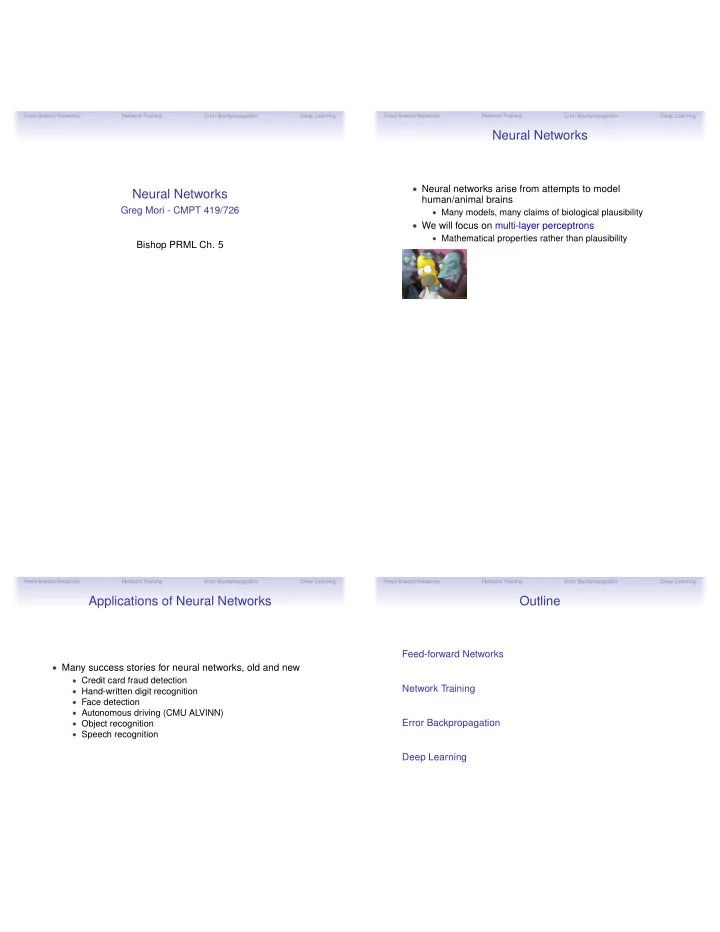
Feed-forward Networks Network Training Error Backpropagation Deep Learning Feed-forward Networks Network Training Error Backpropagation Deep Learning Neural Networks • Neural networks arise from attempts to model Neural Networks human/animal brains Greg Mori - CMPT 419/726 • Many models, many claims of biological plausibility • We will focus on multi-layer perceptrons • Mathematical properties rather than plausibility Bishop PRML Ch. 5 Feed-forward Networks Network Training Error Backpropagation Deep Learning Feed-forward Networks Network Training Error Backpropagation Deep Learning Applications of Neural Networks Outline Feed-forward Networks • Many success stories for neural networks, old and new • Credit card fraud detection Network Training • Hand-written digit recognition • Face detection • Autonomous driving (CMU ALVINN) Error Backpropagation • Object recognition • Speech recognition Deep Learning

Feed-forward Networks Network Training Error Backpropagation Deep Learning Feed-forward Networks Network Training Error Backpropagation Deep Learning Feed-forward Networks Feed-forward Networks • Starting with input x = ( x 1 , . . . , x D ) , construct linear • We have looked at generalized linear models of the form: combinations:   D M � w ( 1 ) ji x i + w ( 1 ) � a j = y ( x , w ) = f w j φ j ( x ) j 0   i = 1 j = 1 These a j are known as activations for fixed non-linear basis functions φ ( · ) • Pass through an activation function h ( · ) to get output z j = h ( a j ) • We now extend this model by allowing adaptive basis • Model of an individual neuron functions, and learning their parameters • In feed-forward networks (a.k.a. multi-layer perceptrons) we let each basis function be another non-linear function of linear combination of the inputs:   M � φ j ( x ) = f . . .   j = 1 from Russell and Norvig, AIMA2e Feed-forward Networks Network Training Error Backpropagation Deep Learning Feed-forward Networks Network Training Error Backpropagation Deep Learning Activation Functions Feed-forward Networks hidden units z M w (1) • Can use a variety of activation functions MD w (2) KM x D • Sigmoidal (S-shaped) y K • Logistic sigmoid 1 / ( 1 + exp ( − a )) (useful for binary outputs inputs classification) y 1 • Hyperbolic tangent tanh x 1 • Radial basis function z j = � i ( x i − w ji ) 2 z 1 w (2) • Softmax 10 x 0 • Useful for multi-class classification z 0 • Identity • Connect together a number of these units into a • Useful for regression feed-forward network (DAG) • Threshold • Above shows a network with one layer of hidden units • Max, ReLU, Leaky ReLU, . . . • Implements function: • Needs to be differentiable* for gradient-based learning   � D (later) � M � � w ( 2 ) w ( 1 ) ji x i + w ( 1 ) + w ( 2 ) y k ( x , w ) = h • Can use different activation functions in each unit kj h   j 0 k 0 j = 1 i = 1

Feed-forward Networks Network Training Error Backpropagation Deep Learning Feed-forward Networks Network Training Error Backpropagation Deep Learning Network Training Parameter Optimization • Given a specified network structure, how do we set its E ( w ) parameters (weights)? • As usual, we define a criterion to measure how well our network performs, optimize against it • For regression, training data are ( x n , t ) , t n ∈ R • Squared error naturally arises: N � { y ( x n , w ) − t n } 2 E ( w ) = w 1 n = 1 w A w B • For binary classification, this is another discriminative w C model, ML: w 2 ∇ E N � • For either of these problems, the error function E ( w ) is y t n n { 1 − y n } 1 − t n p ( t | w ) = nasty n = 1 • Nasty = non-convex N � • Non-convex = has local minima E ( w ) = − { t n ln y n + ( 1 − t n ) ln ( 1 − y n ) } n = 1 Feed-forward Networks Network Training Error Backpropagation Deep Learning Feed-forward Networks Network Training Error Backpropagation Deep Learning Descent Methods Computing Gradients • The function y ( x n , w ) implemented by a network is • The typical strategy for optimization problems of this sort is complicated a descent method: • It isn’t obvious how to compute error function derivatives w ( τ + 1 ) = w ( τ ) + ∆ w ( τ ) with respect to weights • Numerical method for calculating error derivatives, use finite differences: • As we’ve seen before, these come in many flavours ≈ E n ( w ji + ǫ ) − E n ( w ji − ǫ ) ∂ E n • Gradient descent ∇ E ( w ( τ ) ) ∂ w ji 2 ǫ • Stochastic gradient descent ∇ E n ( w ( τ ) ) • Newton-Raphson (second order) ∇ 2 • All of these can be used here, stochastic gradient descent • How much computation would this take with W weights in is particularly effective the network? • Redundancy in training data, escaping local minima • O ( W ) per derivative, O ( W 2 ) total per gradient descent step

Feed-forward Networks Network Training Error Backpropagation Deep Learning Feed-forward Networks Network Training Error Backpropagation Deep Learning Error Backpropagation Chain Rule for Partial Derivatives • Backprop is an efficient method for computing error derivatives ∂ E n ∂ w ji • O ( W ) to compute derivatives wrt all weights • A “reminder” • First, feed training example x n forward through the network, • For f ( x , y ) , with f differentiable wrt x and y , and x and y storing all activations a j differentiable wrt u : • Calculating derivatives for weights connected to output nodes is easy ∂ f ∂ f ∂ u + ∂ f ∂ x ∂ y • e.g. For linear output nodes y k = � = i w ki z i : ∂ u ∂ x ∂ y ∂ u ∂ E n ∂ 1 2 ( y ( n ) , k − t ( n ) , k ) 2 = ( y ( n ) , k − t ( n ) , k ) z ( n ) i = ∂ w ki ∂ w ki • For hidden layers, propagate error backwards from the output nodes Feed-forward Networks Network Training Error Backpropagation Deep Learning Feed-forward Networks Network Training Error Backpropagation Deep Learning Error Backpropagation Error Backpropagation cont. • We can write ∂ E n ∂ = E n ( a j 1 , a j 2 , . . . , a j m ) ∂ w ji ∂ w ji • Introduce error δ j ≡ ∂ E n ∂ a j where { j i } are the indices of the nodes in the same layer as node j ∂ a j ∂ E n = δ j • Using the chain rule: ∂ w ji ∂ w ji ∂ E n = ∂ E n ∂ a j ∂ E n ∂ a k � + • Other factor is: ∂ w ji ∂ a j ∂ w ji ∂ a k ∂ w ji k ∂ a j ∂ � where � = w jk z k = z i k runs over all other nodes k in the same layer as ∂ w ji ∂ w ji node j . k • Since a k does not depend on w ji , all terms in the summation go to 0 ∂ a j ∂ E n = ∂ E n ∂ w ji ∂ a j ∂ w ji

Feed-forward Networks Network Training Error Backpropagation Deep Learning Feed-forward Networks Network Training Error Backpropagation Deep Learning Error Backpropagation cont. Deep Learning • Error δ j can also be computed using chain rule: • Collection of important techniques to improve performance: δ j ≡ ∂ E n ∂ E n ∂ a k � • Multi-layer networks = ∂ a j ∂ a k ∂ a j • Convolutional networks, parameter tying k ���� • Hinge activation functions (ReLU) for steeper gradients δ k • Momentum where � • Drop-out regularization k runs over all nodes k in the layer after node j . • Sparsity • Eventually: • Auto-encoders for unsupervised feature learning � δ j = h ′ ( a j ) w kj δ k • ... k • Scalability is key, can use lots of data since stochastic gradient descent is memory-efficient, can be parallelized • A weighted sum of the later error “caused” by this weight Feed-forward Networks Network Training Error Backpropagation Deep Learning Feed-forward Networks Network Training Error Backpropagation Deep Learning Hand-written Digit Recognition LeNet-5, circa 1998 C3: f. maps 16@10x10 C1: feature maps S4: f. maps 16@5x5 INPUT 6@28x28 32x32 S2: f. maps C5: layer F6: layer OUTPUT 6@14x14 120 10 84 Gaussian connections Full connection Subsampling Subsampling Convolutions Convolutions Full connection • LeNet developed by Yann LeCun et al. • Convolutional neural network • Local receptive fields (5x5 connectivity) • Subsampling (2x2) • MNIST - standard dataset for hand-written digit recognition • Shared weights (reuse same 5x5 “filter”) • Breaking symmetry • 60000 training, 10000 test images