(Very) Brief Introduction to Neural Networks IITP-03 Algorithms for - PowerPoint PPT Presentation
(Very) Brief Introduction to Neural Networks IITP-03 Algorithms for NLP 1 / 31 Learning objectives What are neural networks? What are deep neural networks? How do we train neural networks? What variants of neural network
(Very) Brief Introduction to Neural Networks IITP-03 Algorithms for NLP 1 / 31
Learning objectives ● What are neural networks? ● What are deep neural networks? ● How do we train neural networks? ● What variants of neural network architectures exist, and are good for? ● What are strengths and weaknesses of neural networks? ● How are neural networks used for NLP? 2 / 31
Neural networks ● Network of neurons – Electrically excitable nerve cells ● When we talk about neural nets, we’re actually referring to Artifjcal Neural Networks (ANNs) 3 / 31
Perceptron ● Classifjcation algorithm motivated from a single neuron 4 / 31
Perceptron ● Easy to train, but limited expressivity… ● Specifjcally, could not learn non-linear decision boundaries with a single perceptron – XOR problem 5 / 31
Multilayer perceptrons ● Instead of using elementary input features, fjnd some feature combinations to use as another set of input features – i.e. map to a difgerent feature space! y h 2 =step(-x+y-0.5>0) 1 1 x 0 0 h 1 =step(x-y-0.5>0) 1 1 6 / 31
Multilayer perceptrons ● This is equivalent to stacking layers of perceptrons 1 h 1 x 1 -1 1 -1 out h 2 y 1 -0.5 0.5 -0.5 1 1 ● This is the reason why we sometimes refer to neural network techniques as ‘deep learning’: instead of shallow input-output networks, we use deep networks with multiple ‘hidden’ stacks of layers to automatically recognize features 7 / 31
Multilayer perceptrons ● The nonlinearity at the end of each perceptron output is crucial – E.g. step function, sigmoid, tanh, … ● Without the nonlinearity, stacking whatever number of layers would be equivalent to using just one layer – Product of any number of matrices is simply another matrix 8 / 31
Deep learners are feature extractors ● Each hidden unit in deep neural networks correspond to a combination of features from the lower level ● No need to do explicit feature engineering! 9 / 31
Training MLPs ● For a single layer of perceptrons, training is simple and intuitive – Randomly initialize weights of each unit – For instances where the prediction is wrong, adjust weights of corresponding units by some learning step size ● But how do we ‘propagate’ the errors further back, past the penultimate layer? 10 / 31
Backpropagation ● Computes gradients of the loss function with respect to the network parameters via chain rule ● Independently proposed by various researchers in 1960-70s, but haven’t received much attention until... ● Rumelhart, Hinton and Williams (1986) experimentally shows backpropagation actually works, and defjnes the modern framework 11 / 31
Backpropagation ● Computation graphs are a nice way to represent and understand backpropagation: Forward pass: Compute all the Backward pass: Compute the intermediate values in the graph gradients w.r.t immediate inputs in reverse order ● (In general, you rarely have to implement backpropagation from scratch by yourself...) 12 / 31
Activation functions ● By design, all the computations involved should be difgerentiable for backpropagation ● This implies our choice of nonlinearity becomes somewhat limited: 13 / 31
Deep learners are universal approximators ● It is proven that deep NNs with ‘enough’ number of hidden units and layers can approximate any continuous function ● Of course there are some caveats... 14 / 31
Convolutional NNs ● For data of extensive scales (like images), it is mostly the case that exact locations where local patterns occur do not really matter ● CNNs (LeCun, 1989) use two types of layers to automatically extract local patterns: – Convolutional layer: Identify local patterns with fjlters – Pooling layer: Summarize the result of applying each fjlter for areas, downsampling the input 15 / 31
Convolutional NNs 16 / 31
Recurrent NNs ● What if our data is sequential in nature? – E.g. Acoustic waves, natural language sentences ● In some cases, we cannot afgord to lose the structural information – “It isn’t bad, but not that good” – “It isn’t good, but not that bad” – When word order matters, simply using bag-of-words here is to lose great amount of information 17 / 31
Recurrent NNs ● In feed-forward NNs, computations fmow only forward ● In RNNs, outputs from a hidden layer is fed back to the same layer as input 18 / 31
Recurrent NNs ● RNNs can be multi-layered or bidirectional ● Of course, comes at a price of larger models 19 / 31
Recurrent NNs ● Naturally, RNNs are heavily used for NLP tasks – Document classifjcation – Sequence tagging – Sequence transduction – And so many more... 20 / 31
Gated RNNs ● RNNs are also trained by backpropagation, on the unrolled computation graphs ● However, the multiplicative nature of backpropagation algorithm causes a problem – Same terms are multiplied so many times, the gradients may explode, or worse, vanish ● As a result, despite the promise, simple RNNs cannot capture longer-distance relationships 21 / 31
Gated RNNs ● As a solution, gated architectures use a cell state that works somewhat like a ‘conveyer belt’ – Long Short-T erm Memory (Hochreiter, 1997) ● Again, don’t worry about implementations :) 22 / 31
Word embeddings ● An especially useful neural network technique for NLP tasks ● Dense low-dimensional representation of words (instead of sparse high-dimensional) ● Based on distributional semantics – “You shall know a word by the company it keeps” (J. R. Firth, 1957) – Words that occur in similar contexts have similar representations 23 / 31
Word embeddings ● Word embedding simply refers to the idea of representing a word with dense vectors – We can think of sentence, character, morpheme embeddings as well ● Obtained from some unsupervised tasks like language modeling ● Compared to random initialization, pre- trained word embeddings are known to boost performance of most neural NLP systems by a signifjcant margin 24 / 31
Word embeddings ● Power of distributional representations – Models can ‘notice’ similar words – Sparsity problem can be (partially) resolved – Markov assumption can be relaxed – Allows fmexible generative modeling ● Note that neural methods don’t have to use distribution representations, and vice versa – It’s just that they work together SO well 25 / 31
Word embeddings ● An obligatory example: – king – man + woman = queen ● But are they really learning semantics? 26 / 31
Word embeddings ● Many words are polysemous, and their meanings may vary in difgerent contexts – “He went to the prison cell with his cell phone to extract blood cell samples from inmates” ● Contextual word embeddings like ELMo or BERT can take the context into account – Embeddings are defjned for each word token, not word type – Most of the current state-of-the-art NLP systems are based on BERT 27 / 31
Weaknesses of NNs ● Excessively data-hungry – NNs tend to overfjt, and not generalize well on new instances – Need large amounts of examples to show the ‘impressive’ performance – Naturally, require huge amounts of computational resources ● Highly non-interpretable – In most cases, we have ZERO idea about what each parameter in neural networks actually represents 28 / 31
Some neural net practicalities ● Gradient descent – The gradients obtained from backward passes can be applied by various GD optimizers – e.g. SGD, RMSprop, Adagrad, Adam... ● Mini-batch GD – Between batch GD & online (stochastic) GD – Stable convergence, effjcient computation 29 / 31
Some neural net practicalities ● Weight initialization – T urns out, initializing with random weights without consideration can be very bad – Use initialization techniques like Xavier initialization or Kaiming initialization ● Regularization by dropout – Randomly disabling some units can prevent co-adaptation – Acts as regularization for NNs 30 / 31
Some references ● Great summary on the high-level history of deep learning – https://www.andreykurenkov.com/writing/ ai/a-brief-history-of-neural-nets-and-deep- learning/ ● Blog with lots of introductory NN & ML posts – https://colah.github.io/ 31 / 31
Recommend
More recommend
Explore More Topics
Stay informed with curated content and fresh updates.
