Learning Neural Networks Learning Neural Networks Neural Networks - PowerPoint PPT Presentation

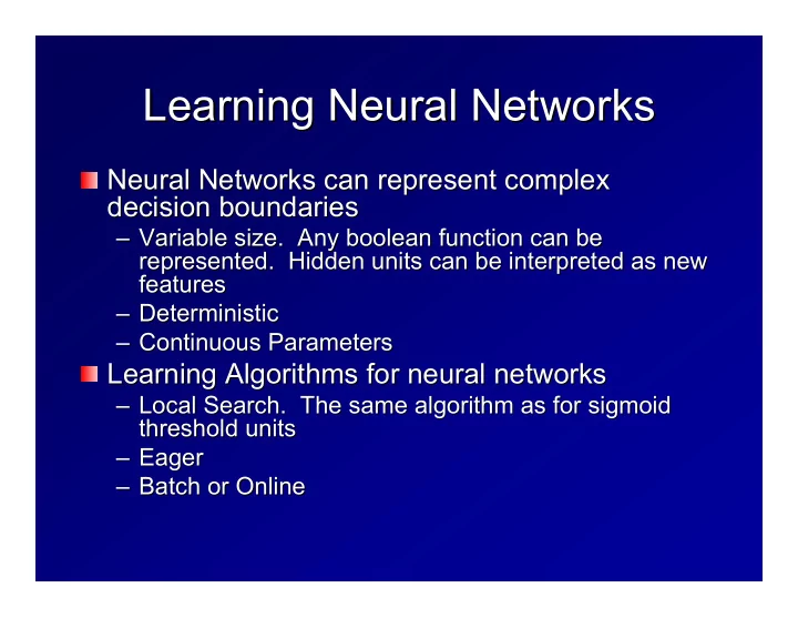
Learning Neural Networks Learning Neural Networks Neural Networks can represent complex Neural Networks can represent complex decision boundaries decision boundaries – Variable size. Any boolean function can be Variable size. Any boolean function can be – represented. Hidden units can be interpreted as new represented. Hidden units can be interpreted as new features features – Deterministic Deterministic – – Continuous Parameters Continuous Parameters – Learning Algorithms for neural networks Learning Algorithms for neural networks – Local Search. The same algorithm as for sigmoid Local Search. The same algorithm as for sigmoid – threshold units threshold units – Eager Eager – – Batch or Online Batch or Online –

Neural Network Hypothesis Space Neural Network Hypothesis Space ŷ W 9 a 6 a 7 a 8 W 6 W 7 W 8 x 1 x 2 x 3 x 4 Each unit a 6 Each unit a 6 , a , a 7 7 , a , a 8 8 , and , and ŷ ŷ computes a sigmoid function of its inputs: computes a sigmoid function of its inputs: σ (W σ (W σ (W σ (W = σ = σ = σ = σ a 6 (W 6 · X) a X) a 7 (W 7 · X) a X) a 8 (W 8 · X) X) ŷ ŷ = (W 9 · A) A) a 6 = 7 = 8 = 6 · 7 · 8 · 9 · where A = [1, a 6 where A = [1, a 6 , a , a 7 7 , a , a 8 8 ] is called the vector of ] is called the vector of hidden unit activitations hidden unit activitations Original motivation: Differentiable approximation to multi- -layer LTUs layer LTUs Original motivation: Differentiable approximation to multi

Representational Power Representational Power Any Boolean Formula Any Boolean Formula – Consider a formula in disjunctive normal form: Consider a formula in disjunctive normal form: – (x 1 ¬ x x 2 ) ∨ ∨ (x (x 2 ∧ x x 4 ) ∨ ∨ ( ( ¬ ¬ x x 3 ∧ x x 5 ) (x 2 ) 4 ) 5 ) 1 ∧ ∧ ¬ 2 ∧ 3 ∧ Each AND can be represented by a hidden unit and the OR can Each AND can be represented by a hidden unit and the OR can be represented by the output unit. Arbitrary boolean functions be represented by the output unit. Arbitrary boolean functions require exponentially- require exponentially -many hidden units, however. many hidden units, however. Bounded functions Bounded functions – Suppose we make the output linear: – Suppose we make the output linear: ŷ ŷ = W = W 9 · A of hidden units. A of hidden units. 9 · It can be proved that any bounded continuous function can be It can be proved that any bounded continuous function can be approximated to arbitrary accuracy with enough hidden units. approximated to arbitrary accuracy with enough hidden units. Arbitrary Functions Arbitrary Functions – Any function can be approximated to arbitrary accuracy with two Any function can be approximated to arbitrary accuracy with two – hidden layers of sigmoid units and a linear output unit. hidden layers of sigmoid units and a linear output unit.

Fixed versus Variable Size Fixed versus Variable Size In principle, a network has a fixed number of parameters In principle, a network has a fixed number of parameters and therefore can only represent a fixed hypothesis and therefore can only represent a fixed hypothesis space (if the number of hidden units is fixed). space (if the number of hidden units is fixed). However, we will initialize the weights to values near However, we will initialize the weights to values near zero and use gradient descent. The more steps of zero and use gradient descent. The more steps of gradient descent we take, the more functions can be gradient descent we take, the more functions can be “reached reached” ” from the starting weights. from the starting weights. “ So it turns out to be more accurate to treat networks as So it turns out to be more accurate to treat networks as having a variable hypothesis space that depends on the having a variable hypothesis space that depends on the number of steps of gradient descent number of steps of gradient descent

Backpropagation: Gradient Backpropagation: Gradient Descent for Multi- -Layer Networks Layer Networks Descent for Multi It is traditional to train neural networks to minimize the squared It is traditional to train neural networks to minimize the squar ed error. This is really a mistake— —they should be trained to maximize they should be trained to maximize error. This is really a mistake the log likelihood instead. But we will study the MSE first. the log likelihood instead. But we will study the MSE first. y = σ ( W 9 · [1 , σ ( W 6 · X ) , σ ( W 7 · X ) , σ ( W 9 · X )]) ˆ J i ( W ) = 1 y i − y i ) 2 2(ˆ We must apply the chain rule many times to compute the gradient We must apply the chain rule many times to compute the gradient We will number the units from 0 to U and index them by u u and and v v . . We will number the units from 0 to U and index them by w v,u will be the weight connecting unit u u to unit to unit v. v. (Note: This seems (Note: This seems w v,u will be the weight connecting unit backwards. It is the u u th input to node th input to node v v .) .) backwards. It is the

Derivation: Output Unit Derivation: Output Unit Suppose w w 9,6 is a component of W W 9 , the Suppose 9,6 is a component of 9 , the output weight vector, connecting it from a a 6 . output weight vector, connecting it from 6 . ∂ J i ( W ) 1 ∂ y i − y i ) 2 = 2(ˆ ∂ w 9 , 6 ∂ w 9 , 6 1 ∂ = 2 · 2 · (ˆ y i − y i ) · ( σ ( W 9 · A i ) − y i ) ∂ w 9 , 6 ∂ = (ˆ y i − y i ) · σ ( W 9 · A i )(1 − σ ( W 9 · A i )) · W 9 · A i ∂ w 9 , 6 = (ˆ y i − y i )ˆ y i (1 − ˆ y i ) · a 6

The Delta Rule The Delta Rule Define Define δ 9 = (ˆ y i − y i )ˆ y i (1 − ˆ y i ) then then ∂ J i ( W ) = (ˆ y i − y i )ˆ y i (1 − ˆ y i ) · a 6 ∂ w 9 , 6 = δ 9 · a 6

Derivation: Hidden Units Derivation: Hidden Units ∂ J i ( W ) ∂ = (ˆ y i − y i ) · σ ( W 9 · A i )(1 − σ ( W 9 · A i )) · W 9 · A i ∂ w 6 , 2 ∂ w 6 , 2 ∂ = δ 9 · w 9 , 6 · σ ( W 6 · X ) ∂ w 6 , 2 ∂ = δ 9 · w 9 , 6 · σ ( W 6 · X )(1 − σ ( W 6 · X )) · ( W 6 · X ) ∂ w 6 , 2 = δ 9 · w 9 , 6 a 6 (1 − a 6 ) · x 2 Define δ 6 = δ 9 · w 9 , 6 a 6 (1 − a 6 ) and rewrite as ∂ J i ( W ) = δ 6 x 2 . ∂ w 6 , 2

Networks with Multiple Output Units Networks with Multiple Output Units ŷ 1 ŷ 2 a 7 a 8 a 6 1 W 6 W 7 W 8 1 x 1 x 2 x 3 x 4 We get a separate contribution to the gradient from each We get a separate contribution to the gradient from each output unit. output unit. Hence, for input- -to to- -hidden weights, we must sum up the hidden weights, we must sum up the Hence, for input contributions: contributions: 10 X δ 6 = a 6 (1 − a 6 ) w u, 6 δ u u =9

The Backpropagation Algorithm The Backpropagation Algorithm Forward Pass. Compute . Compute a a u and ŷ ŷ v for hidden units u u and and Forward Pass u and v for hidden units output units v v . . output units ε v . Compute ε Compute Errors. Compute = ( ŷ ŷ v – y y v ) for each output Compute Errors v = ( v – v ) for each output unit v v unit δ u ∑ v δ v . Compute δ ) ∑ v,u δ Compute Output Deltas. Compute = a a u (1 – – a a u w v,u Compute Output Deltas u = u (1 u ) v w v Compute Gradient. . Compute Gradient ∂ J i – Compute for input – Compute for input- -to to- -hidden weights. hidden weights. = δ u x ij ∂ w u,j ∂ J i – Compute for hidden – Compute for hidden- -to to- -output weights. output weights. = δ v a iu ∂ w v,u Take Gradient Step. . Take Gradient Step W := W − η ∇ W J ( x i )

Proper Initialization Proper Initialization Start in the “ “linear linear” ” regions regions Start in the – keep all weights near zero, so that all sigmoid units are in the keep all weights near zero, so that all sigmoid units are in their ir – linear regions. This makes the whole net the equivalent of one linear regions. This makes the whole net the equivalent of one linear threshold unit— —a very simple function. a very simple function. linear threshold unit Break symmetry. Break symmetry. – Ensure that each hidden unit has different input weights so that Ensure that each hidden unit has different input weights so that – the hidden units move in different directions. the hidden units move in different directions. Set each weight to a random number in the range Set each weight to a random number in the range 1 [ − 1 , +1] × √ fan-in . where the “ “fan fan- -in in” ” of weight of weight w w v,u is the number of inputs where the v,u is the number of inputs to unit v v . . to unit

Batch, Online, and Online with Batch, Online, and Online with Momentum Momentum Batch. Sum the for each example . Sum the for each example i i . . Batch ∇ W J ( x i ) Then take a gradient descent step. Then take a gradient descent step. Online. Take a gradient descent step with each . Take a gradient descent step with each Online as it is computed. as it is computed. ∇ W J ( x i ) Momentum. Maintain an exponentially . Maintain an exponentially- -weighted weighted Momentum moved sum of recent moved sum of recent ∆ W ( t +1) := µ ∆ W ( t ) + ∇ W J ( x i ) W ( t +1) := W ( t ) − η ∆ W ( t +1) µ are in the range [0.7, 0.95] Typical values of µ are in the range [0.7, 0.95] Typical values of