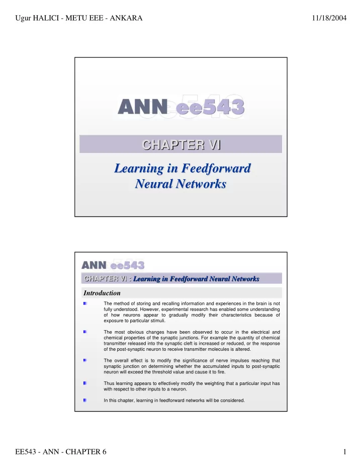
CHAPTER VI VI CHAPTER Learning in Feedforward Feedforward - - PDF document

Ugur HALICI - METU EEE - ANKARA 11/18/2004 EE543 - ANN - CHAPTER 6 1

Learning in Learning in Feedforward Feedforward Neural Networks Neural Networks CHAPTER CHAPTER VI VI

CHAPTER CHAPTER VI : VI : Learning in Learning in Feedforward Feedforward Neural Networks Neural Networks Introduction

The method of storing and recalling information and experiences in the brain is not fully understood. However, experimental research has enabled some understanding

• f how neurons appear to gradually modify their characteristics because of

exposure to particular stimuli. The most obvious changes have been observed to occur in the electrical and chemical properties of the synaptic junctions. For example the quantity of chemical transmitter released into the synaptic cleft is increased or reduced, or the response

• f the post-synaptic neuron to receive transmitter molecules is altered.

The overall effect is to modify the significance of nerve impulses reaching that synaptic junction on determining whether the accumulated inputs to post-synaptic neuron will exceed the threshold value and cause it to fire. Thus learning appears to effectively modify the weighting that a particular input has with respect to other inputs to a neuron. In this chapter, learning in feedforward networks will be considered.

Ugur HALICI - METU EEE - ANKARA 11/18/2004 EE543 - ANN - CHAPTER 6 2

CHAPTER CHAPTER VI : VI : Learning in Learning in Feedforward Feedforward Neural Networks Neural Networks 6.1. Perceptron Convergence Procedure

• Perceptron was introduced by Frank Rosenblatt in the late 1950's (Rosenblatt, 1958) with

a learning algorithm on it.

• Perceptron may have continuous valued inputs.
• It works in the same way as the formal artificial neuron defined previously.
• Its activation is determined by equation:

a=wTu + θ (6.1.1)

• Moreover, its output function is:

(6.1.2) having value either +1 or -1. ⎩ ⎨ ⎧ < − ≥ + = a for a for a f 1 1 ) (

CHAPTER CHAPTER VI : VI : Learning in Learning in Feedforward Feedforward Neural Networks Neural Networks 6.1. Perceptron Convergence Procedure

Figure 6.1. Perceptron

Ugur HALICI - METU EEE - ANKARA 11/18/2004 EE543 - ANN - CHAPTER 6 3

CHAPTER CHAPTER VI : VI : Learning in Learning in Feedforward Feedforward Neural Networks Neural Networks 6.1. Perceptron Convergence Procedure

• Now, consider such a perceptron in N dimensional space (Figure 6.1), the equation

wTu +θ = 0 (6.1.3) that is w1u1+w2u2+...+wN uN + θ = 0 (6.1.4) defines a hyperplane.

• This hyperplane divides the input space into two parts such that at one side, the

perceptron has output value +1, and in the other side, it is -1.

CHAPTER CHAPTER VI : VI : Learning in Learning in Feedforward Feedforward Neural Networks Neural Networks 6.1. Perceptron Convergence Procedure

• A perceptron can be used to decide whether an input vector belongs to one of the two

classes, say classes A and B.

• The decision rule may be set as to respond as class A if the output is +1 and as class B if

the output is -1.

• The perceptron forms two decision regions separated by the hyperplane.
• The equation of the boundary hyperplane depends on the connection weights and

threshold.

Ugur HALICI - METU EEE - ANKARA 11/18/2004 EE543 - ANN - CHAPTER 6 4

CHAPTER CHAPTER VI : VI : Learning in Learning in Feedforward Feedforward Neural Networks Neural Networks 6.1. Perceptron Convergence Procedure

Example 6.1: When the input space is two-dimensional then the equation w1u1+w2u2 + θ= 0 (6.1.5) defines a line as shown in the Figure 6.2. This line divides the space of input variables u1 and u2, which is a plane, into to two separate parts. In the given figure the elements of the classes A and B lies on the different sides of the line. Figure 6.2. Perceptron output defines a hyperplane that divides input space into two separate subspaces

A

u1 u2 u1w1 + u1w1 + θ = 0 x u1 u2 1 θ w1 w2

B

CHAPTER CHAPTER VI : VI : Learning in Learning in Feedforward Feedforward Neural Networks Neural Networks 6.1. Perceptron Convergence Procedure

• Connection weights and the threshold in a perceptron can be fixed or adapted by using a

number of different algorithms.

• The original perceptron convergence procedure developed by [Rosenblatt, 1959] for

adjusting weights is provided in the following.

Ugur HALICI - METU EEE - ANKARA 11/18/2004 EE543 - ANN - CHAPTER 6 5

CHAPTER CHAPTER VI : VI : Learning in Learning in Feedforward Feedforward Neural Networks Neural Networks 6.1. Perceptron Convergence Procedure

Step 1: Initialize weights and threshold Set each wj(0), for j=0,1,2,..,N, in w(0) to small random values. Here w=w(t) is the weight vector at iteration time t and the component w0=θ corresponds to the bias. Step 2. Present New Input and Desired output: Present new continuous valued input vector uk along with the desired output yk, such that: Step 3. Calculate actual output xk=f(wTuk) Step 4. Adapt weights w(t+1)=w(t)+η (yk-xk(t)) uk where η is a positive gain fraction less than 1 Step 5. Repeat steps 2-4 until no error occurs y if input is from class A if input is from class B

k = +

− 1 1

CHAPTER CHAPTER VI : VI : Learning in Learning in Feedforward Feedforward Neural Networks Neural Networks 6.1. Perceptron Convergence Procedure

Example 6.2: Figure 6.3 demonstrates how the line defined by the perceptrons parameters is shifted in time as the weights are updated. Although it is not able to separate the classes A and B with the initial weights assigned at time t=0, it manages to separate them at the end. Figure 6.3. Perceptron convergence

A

u1 u2 x u1 u2 1 θ w1 w2

B

t=0 t=1 t=k ...

Ugur HALICI - METU EEE - ANKARA 11/18/2004 EE543 - ANN - CHAPTER 6 6

CHAPTER CHAPTER VI : VI : Learning in Learning in Feedforward Feedforward Neural Networks Neural Networks 6.1. Perceptron Convergence Procedure

• In [Rosenblatt, 1959] it is proved that if the inputs presented from the two classes are

separable, that is they fall on opposite sides of some hyperplane, then the perceptron convergence procedure always converges in time. Furthermore, it positions the final decision hyperplane such that it separates the samples of class A from those of class B. Figure 6.4. (a) Overlapping distributions (b) non linearly separable distribution One problem with the perceptron convergence procedure is that decision boundary may oscillate continuously when the distributions overlap or the classes are not linearly separable (Figure 6.4).

A

u1 u2

B A

u1 u2

B

CHAPTER CHAPTER VI : VI : Learning in Learning in Feedforward Feedforward Neural Networks Neural Networks

Figure 6.5. Types of regions that can be formed by single and multi-layer perceptrons (Adapted from Lippmann 89) A

A B B

STRUCTURE TYPES OF DECISION REGIONS EXCLUSIVE OR PROBLEM MOST GENERAL REGION SHAPES

B B B B

B B B B A A

A A A A A

Ugur HALICI - METU EEE - ANKARA 11/18/2004 EE543 - ANN - CHAPTER 6 7

CHAPTER CHAPTER VI : VI : Learning in Learning in Feedforward Feedforward Neural Networks Neural Networks 6.2 LMS Learning Rule

• A modification to the perceptron convergence procedure forms the Least Mean Square

(LMS) solution for the case that the classes are not separable.

• This solution minimizes the mean square error between the desired output and the actual
• utput of the processing element.
• The LMS algorithm was first proposed for Adaline (Adaptive Linear Element) in [Widrow

and Hoff 60].

CHAPTER CHAPTER VI : VI : Learning in Learning in Feedforward Feedforward Neural Networks Neural Networks 6.2 LMS Learning Rule

• The structure of Adaline is shown in the Figure 6.6. The part of the Adaline that executes

the summation is called Adaptive Linear Combiner Figure 6.6 Adaline

Ugur HALICI - METU EEE - ANKARA 11/18/2004 EE543 - ANN - CHAPTER 6 8

CHAPTER CHAPTER VI : VI : Learning in Learning in Feedforward Feedforward Neural Networks Neural Networks 6.2 LMS Learning Rule

The output function of the Adaline can be represented by the identity function as: f(a)=a (6.2.1)

• So the output can be written in terms of input and weights as:

(6.2.2) where the bias is implemented via a connection to a constant input u0, which means the input vector and the weight vector are of space R(N+1) instead of RN.

• The output equation of Adaline can be written as:

x=wTu (6.2.3) where w and u are weight and input vectors respectively having dimension N+1. x f a w u

j j j N

= =

=

∑

( )

CHAPTER CHAPTER VI : VI : Learning in Learning in Feedforward Feedforward Neural Networks Neural Networks 6.2 LMS Learning Rule

• Suppose that we have a set of input vectors uk, k=1..K, each having its own desired
• utput value yk.
• The performance of the Adaline for a given input value uk can be defined by considering

the difference between the desired output yk and the actual output xk, which is called error and denoted as ε.

• Therefore, the error for the input uk is as follows:

εk=yk-xk=yk-wTuk (6.2.4)

• The aim of the LMS learning is to adjust the weights through a training set {(uk,yk)},

k=1..K, such that the mean of the square of the errors is minimum.

• The mean square error is defined as:

(6.2.5) where the notation <.> denotes the mean value.

∑

= ∞ →

>= <

K k k K k k 1 2 1 2

) ( lim ) ( ε ε

Ugur HALICI - METU EEE - ANKARA 11/18/2004 EE543 - ANN - CHAPTER 6 9

CHAPTER CHAPTER VI : VI : Learning in Learning in Feedforward Feedforward Neural Networks Neural Networks 6.2 LMS Learning Rule

The mean square error can be rewritten as: (6.2.6) where T denotes transpose and x is the outer vector product.

• Defining input correlation matrix R and a vector P as

(6.2.7) (6.2.8) results in: (6.2.9)

• The optimum value w* for the weight vector corresponding to the minimum of the mean

squared error can be obtained by evaluating the gradient of e(w). < >=< − > ( ) ( ) ε k

k k

y

2 2

w u

T

w u w u u w > < − > × < + > =<

T T k k k k k

y y 2 ) (

2

R u u u u =< × > = < >

k k k k T

P u =< > yk

k

e( ) ( ) ( ) w w R w P w =< >=< > + − εk

k

y

2 2

2

T T

CHAPTER CHAPTER VI : VI : Learning in Learning in Feedforward Feedforward Neural Networks Neural Networks 6.2 LMS Learning Rule

• The point which makes the gradient zero gives us the value of w*. That is:

(6.2.10)

• Here, the gradient is

(6.2.11) and it is a vector extending in the direction of the greatest rate of change.

• The gradient of a function evaluated at some point is zero if the function has a maximum
• r minimum at that point.
• The error function is of the second degree. So it is a paraboloid and it has a single

minimum at point w*. ∇ = = − =

= = ∗

∗ ∗

e e ( ) ( ) w w w Rw P

w w w w

∂ ∂ 2 2 ∇ = e

e e e

( ) ... w

∂ ∂ ∂ ∂ ∂ ∂ w w wn

1 2

T

Ugur HALICI - METU EEE - ANKARA 11/18/2004 EE543 - ANN - CHAPTER 6 10

CHAPTER CHAPTER VI : VI : Learning in Learning in Feedforward Feedforward Neural Networks Neural Networks 6.2 LMS Learning Rule

• When we set the gradient of the mean square error to zero, this implies that

Rw*=P (6.2.12) and then w*=R-1P (6.2.13)

CHAPTER CHAPTER VI : VI : Learning in Learning in Feedforward Feedforward Neural Networks Neural Networks 6.3 Steepest Descent Algorithm.

• The analytical calculation of the optimum weight vector for a problem is rather difficult in

general.

• Not only does the matrix manipulation get cumbersome for the large dimensions, but also

each component of R and P itself is an expectation value.

• Thus, explicit calculations of R and P require knowledge of the statistics of the input

signal [Freeman 91].

• A better approach would be to let the Adaline Linear Combiner to find the optimum

weights by itself through a search over the error surface.

Ugur HALICI - METU EEE - ANKARA 11/18/2004 EE543 - ANN - CHAPTER 6 11

CHAPTER CHAPTER VI : VI : Learning in Learning in Feedforward Feedforward Neural Networks Neural Networks 6.3 Steepest Descent Algorithm.

• Instead of having a purely random search, some intelligence is added to the procedure

such that the weight vector is changed by considering the gradient of e(w) iteratively [Widrow 60], according to formula known as delta rule: w(t+1)=w(t)+∆w(t) (6.3.1) where ∆w(t)=-η∇e(w(t)) (6.3.2) In the above formula η is a small positive constant.

CHAPTER CHAPTER VI : VI : Learning in Learning in Feedforward Feedforward Neural Networks Neural Networks 6.3 Steepest Descent Algorithm.

• For the real valued scalar function e(w)
• n a vector space w∈RN, the gradient

e(w) gives the direction of the steepest upward slope, so the negative of the gradient is the direction of the steepest

• descent. This fact is demonstrated in

Figure 6.7 for a parabolic error surface on two dimensions.

• In Section 6.2 we have considered the

linear output function in the derivation of the optimum weight w* for the minimum

• error. However in the general case, we

should consider any nonlinearity f(.) at the

• utput of the neuron. It should be noted

that in such a case the error surface is no more a paraboloid, so it may have several local minima. Figure 6.7 Direction of the steepest gradient descent on the paraboloid error surface on two- dimensional weight space. Only the equpotential curves of the error surface is shown instead of the 3D-error surface.

. minimum

Ugur HALICI - METU EEE - ANKARA 11/18/2004 EE543 - ANN - CHAPTER 6 12

CHAPTER CHAPTER VI : VI : Learning in Learning in Feedforward Feedforward Neural Networks Neural Networks 6.3 Steepest Descent Algorithm.

• For an input uk applied at time t, (εk(t))2 can be used as an approximation to <ε(k)2>, where

ε k(t)=yk-f(ak)=yk-f(w(t)Tuk) (6.3.3)

• Therefore, we obtain:

∇<(ε k)2> ~ ∇(ε k(t))2 = ∇(yk-f(ak))2 (6.3.4)

• With a differentiable function f(.) having derivative f'(.), it becomes

∇(yk-f(a))2= -2 εk (t) f ' (a) ∇ a (6.3.5)

CHAPTER CHAPTER VI : VI : Learning in Learning in Feedforward Feedforward Neural Networks Neural Networks 6.3 Steepest Descent Algorithm.

• Since

∇ak= ∇ w(t)Tuk=uk (6.3.6) the weight update formula becomes: w(t+1)=w(t)+2ηεk(t) f'(a)uk. (6.3.7)

• Notice that for Adaline's linear output function:

f ' (a)=1 (6.3.8)

• For sigmoid function it is:

(6.3.9) ′ = + = −

−

f a a e T f a f a

a T

( ) ( ) ( )( ( ))

/

∂ ∂ 1 1 1 1

Ugur HALICI - METU EEE - ANKARA 11/18/2004 EE543 - ANN - CHAPTER 6 13

CHAPTER CHAPTER VI : VI : Learning in Learning in Feedforward Feedforward Neural Networks Neural Networks 6.3 Steepest Descent Algorithm.

Step 1: Apply an input vector uk with an desired output value yk to the neuron's input Step 2: By considering uk and using the current value of the weight vector determine the value of the activation vector ak: ak=w(t)Tuk Step 3: Determine the value of the derivative of the output function using the current value

• f activation ak, that is:

Step 4: Determine the value of error εk(t) as: ε k(t)= yk-f(ak) Step 5: Update the weight vector with respect to following update formula w(t+1)=w(t)+2η f'(ak) ε k(t)uk Step 6: Repeat steps 1-5 until < εk(t)> reduces to an acceptable level.

k a a k

a a f a f

=

= ∂ ∂ ) ( ) ( '

CHAPTER CHAPTER VI : VI : Learning in Learning in Feedforward Feedforward Neural Networks Neural Networks 6.3 Steepest Descent Algorithm.

The parameter η in the algorithm determines the stability and the speed of convergence of the weight vector towards the minimum error value. The value of η should be tuned well. If it is chosen too small this effects considerably the convergence time. On the other hand, if changes are too large, the weight vector may wander around the minimum as shown in the Figure 6.8, without being able to reach it. Figure 6.8. Inappropriate value of learning rate may cause oscillations in the weight values without convergence

Ugur HALICI - METU EEE - ANKARA 11/18/2004 EE543 - ANN - CHAPTER 6 14

CHAPTER CHAPTER VI : VI : Learning in Learning in Feedforward Feedforward Neural Networks Neural Networks 6.3 Steepest Descent Algorithm.

• Notice that, the iterative weight update by the delta rule is derived by assuming constant

uk.

• Therefore, it tends to minimize the error with respect to applied uk.
• In fact, we require the average error, that is:

(6.3.10) to be minimum

• This implies that

(6.3.11)

∑ ∑

= =

= =

K k j k k K K k j k K j

w w w

1 1 1 2 1

2 ) ( ∂ ∂ε ε ∂ ε ∂ ∂ ∂e

∑

=

>= =<

K k k K k 1 2 1 2

) ( ) ( ε ε e

CHAPTER CHAPTER VI : VI : Learning in Learning in Feedforward Feedforward Neural Networks Neural Networks 6.3 Steepest Descent Algorithm.

• Therefore, the net change in wj after one complete cycle of pattern presentation is

expected to be: (6.3.12)

• However, this would be true that if the weights are not updated along a cycle, but only at

the end.

• By changing the weights as each pattern is presented, we depart to some extend from

the gradient descent in e.

• Nevertheless, provided the learning rate is sufficiently small, this departure will be

negligible and the delta rule will implement a very close approximation to gradient descent in mean squared error [Freeman 91].

∑

=

− = +

K k k k j j

wj K t w K t w

1

2 1 ) ( ) ( ∂ ε ∂ ε η

Ugur HALICI - METU EEE - ANKARA 11/18/2004 EE543 - ANN - CHAPTER 6 15

CHAPTER CHAPTER VI : VI : Learning in Learning in Feedforward Feedforward Neural Networks Neural Networks 6.4. The Backpropagation Algorithm : Single Layer Network

• Consider a single layer multiple output

network as shown in the Figure 6.9.

• Here, we still have N inputs denoted uj,

j=1..N, but M processing elements whose activations and outputs are denoted as ai and xi , i=1..M respectively.

• wji is used to denote the strength of the

connection from the jth input to the ith processing element.

• In vector notation wji is the jth component
• f weight vector wi, while uj is the jth

component of the input vector u.

1 2 j N

x u u u u

i

x

2

x

M

x input layer

• utput layer

=1 1

u

w

ji

Figure 6.9. Single Layer Multiple

• utput network

CHAPTER CHAPTER VI : VI : Learning in Learning in Feedforward Feedforward Neural Networks Neural Networks 6.4. The Backpropagation Algorithm : Single Layer Network

• Let uk and yk to represent the kth input sample and the corresponding desired output

vector respectively

• Let the error observed at the output i, when uk is applied at the input, be

(6.4.1)

• If the error is to be written in terms of the input vector uk

and the weights wi, we obtain (6.4.2) ε i

k i k i k

y x = − ε i

k i k i k

y f = − ( ) w u

T

1 2 j N

x u u u u

i

x

2

x

M

x input layer

• utput layer

=1 1

u

w

ji

Ugur HALICI - METU EEE - ANKARA 11/18/2004 EE543 - ANN - CHAPTER 6 16

CHAPTER CHAPTER VI : VI : Learning in Learning in Feedforward Feedforward Neural Networks Neural Networks 6.4. The Backpropagation Algorithm : Single Layer Network

• If we take partial derivative with respect to wji by applying the chain rule

(6.4.3) where (6.4.4) and (6.4.5) we obtain (6.4.6)

ji k i k i k i ji k i

w x x w ∂ ∂ ∂ ε ∂ ∂ ε ∂ = 1 − =

k i k i

x ∂ ε ∂ ∂ ∂ x w f a u

i k ji i k j k

= ′( ) ∂ε ∂

k ij k j k

w f a u = − ′( )

CHAPTER CHAPTER VI : VI : Learning in Learning in Feedforward Feedforward Neural Networks Neural Networks 6.4. The Backpropagation Algorithm : Single Layer Network

• If we define the total output error for input uk as the sum of the square of the errors at

each neuron output, that is: (6.4.7) then partial derivative of the total error with respect to wji when uk is applied at the input can be written as: (6.4.8) which is (6.4.9) ek

i k i m

=

=

∑

1 2

2 1

( ) ε ∂ ∂ ∂ ∂ ε ∂ε ∂ e e

k ji k i k i k ji

w w = ∂ ∂ ε ek

ji i k k j

w f a u = − ′( )

Ugur HALICI - METU EEE - ANKARA 11/18/2004 EE543 - ANN - CHAPTER 6 17

CHAPTER CHAPTER VI : VI : Learning in Learning in Feedforward Feedforward Neural Networks Neural Networks 6.4. The Backpropagation Algorithm : Single Layer Network

• By defining

(6.4.10) it can be reformulated as (6.4.11) δ ε

i k i k k

f a = ′( )

k j k i ji k

u w δ ∂ ∂ − = e

CHAPTER CHAPTER VI : VI : Learning in Learning in Feedforward Feedforward Neural Networks Neural Networks 6.4. The Backpropagation Algorithm : Single Layer Network

• For the error to be minimum, the gradient of the total error with respect to the weights

should be (6.4.12) where 0 is the vector having N.M entries each having value zero.

• In other words, it should be satisfied:

(6.4.13) ∇ = ek ∂ ∂ ek

ji

w for j 1 N i 1 M = = = .. , ..

Ugur HALICI - METU EEE - ANKARA 11/18/2004 EE543 - ANN - CHAPTER 6 18

CHAPTER CHAPTER VI : VI : Learning in Learning in Feedforward Feedforward Neural Networks Neural Networks 6.4. The Backpropagation Algorithm : Single Layer Network

• In order to reach the minimum of the total error, without solving the above equation, we

apply the delta rule in the same way explained for the steepest descent algorithm: w(t+1)=w(t)-∇ek (6.4.14) in which (6.4.15) that is (6.4.16) M i N j for w t w t w

ji k ji ji

.. 1 , .. 1 ) ( ) 1 ( = = − = + ∂ ∂ η e M i N j for u t w t w

k j k i ji ji

.. 1 , .. 1 ) ( ) 1 ( = = + = + ηδ

CHAPTER CHAPTER VI : VI : Learning in Learning in Feedforward Feedforward Neural Networks Neural Networks 6.4. The Backpropagation Algorithm : Multi Layer Network

• Now assume that another layer of neurons

is connected to the input side of the output layer.

• Therefore we have the input, hidden and

the output layers as shown in Figure 6.10. In order to discriminate between the elements of the hidden and output layers we will use the subscripts L and o respectively.

• Furthermore, we will use h as the index on

the hidden layer elements, while still using index j and i for the input and output layers respectively. Figure 6.10 Multilayer network

Ugur HALICI - METU EEE - ANKARA 11/18/2004 EE543 - ANN - CHAPTER 6 19

CHAPTER CHAPTER VI : VI : Learning in Learning in Feedforward Feedforward Neural Networks Neural Networks 6.4. The Backpropagation Algorithm : Multi Layer Network

• In such a network, the output value of ith neuron of output layer can be written as:

(6.4.17) where being the vector of output values at hidden layer that is connected as input to the output layer. The value of the hth element in xL

k is determined by the equation:

(6.4.18)

• Notice that

(6.4.19) ) (

k L

• i
• k
• i

f x x w

T

= x L

k

) (

k h L k h

L L

f x u w

T

=

k j N j L jh k L h

u w

∑

=

=

1 Tu

w

CHAPTER CHAPTER VI : VI : Learning in Learning in Feedforward Feedforward Neural Networks Neural Networks 6.4. The Backpropagation Algorithm : Multi Layer Network

• The partial derivative of the output of a neuron io of output layer with respect to hidden

layer weight wjhL can be determined by applying the chain rule (6.4.20)

• By using Eq. (6.4.17) and (6.4.19) this can be written as

(6.4.21)

L ij k L h k L h k

• i

L jh k

• i

w x x x w x ∂ ∂ ∂ ∂ ∂ ∂ = ) ) ( ( ) ) ( (

k j k h i h k i jh k i

u a f w a f w x

L L

• L
• L
• ′

′ = ∂ ∂

Ugur HALICI - METU EEE - ANKARA 11/18/2004 EE543 - ANN - CHAPTER 6 20

CHAPTER CHAPTER VI : VI : Learning in Learning in Feedforward Feedforward Neural Networks Neural Networks 6.4. The Backpropagation Algorithm : Multi Layer Network

• Then the partial derivative of the total error

(6.4.22) with respect to the hidden layer weight can be written as (6.4.23)

2 1 2 1 2 1 2 1

) ( ) (

k i M i k i M i k i k

• x

y − = =

∑ ∑

= =

ε e wjhL

k j k h i h k i M i k i h j k

u a f w a f w

L L

• L
• L

) ( ) (

1

′ ′ − = ∑

=

ε ∂ ∂ e

CHAPTER CHAPTER VI : VI : Learning in Learning in Feedforward Feedforward Neural Networks Neural Networks 6.4. The Backpropagation Algorithm : Multi Layer Network

• It can be reformulated as

(6.4.24)

• When defined

(6.4.25) it becomes (6.4.26).

k j k h i h M i k i h j k

u a f w w

L L

• L
• L

) (

1

′ − = ∑

=

δ ∂ ∂ e δ δ

h k h k i k i M h i

L L L

• L o

f a w = ′

=

∑

( )

1

∂ ∂ δ ek

j h h k j

w u

L L

= −

Ugur HALICI - METU EEE - ANKARA 11/18/2004 EE543 - ANN - CHAPTER 6 21

CHAPTER CHAPTER VI : VI : Learning in Learning in Feedforward Feedforward Neural Networks Neural Networks 6.4. The Backpropagation Algorithm : Multi Layer Network

• Therefore, the weight update rule for the hidden layer

(6.4.27) can be reformulated in analogy with the weight update rule of the output layer, as (6.4.28) w t w t w

j h j h k jh

L L L

( ) ( ) + = − 1 η ∂ ∂ e w t w t u

j h j h h k j

L L L

( ) ( ) + = + 1 ηδ

CHAPTER CHAPTER VI : VI : Learning in Learning in Feedforward Feedforward Neural Networks Neural Networks 6.4. The Backpropagation Algorithm : Multi Layer Network

• This weight update rule may be generalized for the networks having several hidden

layers as: (6.4.29) where L and (L-1) are used to denote any hidden layer and its previous layer respectively.

• Furthermore,

(6.4.30) where NL is the number of neurons at layer L. w t w t x

j h j h h k j

L L L L L L ( ) ( ) ( )

( ) ( )

− − −

+ = +

1 1 1

1 ηδ

L L L L L L L L

h j N h k h k j k j

w a f

) 1 ( ) 1 ( 1 ) 1 (

1

) (

− − − −

∑

=

′ = δ δ

Ugur HALICI - METU EEE - ANKARA 11/18/2004 EE543 - ANN - CHAPTER 6 22

CHAPTER CHAPTER VI : VI : Learning in Learning in Feedforward Feedforward Neural Networks Neural Networks 6.4. The Backpropagation Algorithm : Multi Layer Network

Step 0. Initialize weights: to small random values; Step 1. Apply a sample: apply to the input a sample vector uk having desired output vector yk; Step 2. Forward Phase: Starting from the first hidden layer and propagating towards the output layer: 2.1. Calculate the activation values for the units at layer L as: 2.1.1. If L-1 is the input layer 2.1.2. If L-1 is a hidden layer 2.2. Calculate the output values for the units at layer L as: in which use index io instead of hL if it is an output layer

∑

=

=

N j k j h j k h

u w a

L L

∑

− − − −

=

=

1 1 ) 1 ( ) 1 ( L L L L L L

N j k j h j k h

x w a ) (

k L h L k L h

a f x =

CHAPTER CHAPTER VI : VI : Learning in Learning in Feedforward Feedforward Neural Networks Neural Networks 6.4. The Backpropagation Algorithm : Multi Layer Network

Step 4. Output errors: Calculate the error terms at the output layer as: Step 5. Backward Phase Propagate error backward to the input layer through each layer L using the error term in which, use io instead of i(L+1) if L+1 is an output layer; ) ( ) (

k

• i
• k
• i

k

• i

k

• i

a f x y ′ − = δ

∑

+ = + + +

′ =

1 1 1 ) 1 ( ) 1 (

) (

L N L i k L i L h k L i k L h L k L h

w a f δ δ

Ugur HALICI - METU EEE - ANKARA 11/18/2004 EE543 - ANN - CHAPTER 6 23

CHAPTER CHAPTER VI : VI : Learning in Learning in Feedforward Feedforward Neural Networks Neural Networks 6.4. The Backpropagation Algorithm : Multi Layer Network

Step 6. Weight update: Update weights according to the formula

• Step7. Repeat steps 1-6 until the stop criterion is satisfied, which may be chosen as the

mean of the total error is sufficiently small.

k j k h h j h j

L L L L L L

x t w t w

) 1 ( ) 1 ( ) 1 (

) ( ) 1 (

− − −

+ = + ηδ > − >=< <

∑

= 2 1 2 1

) (

k i M i k i k

• x

y e