Machine Learning - MT 2016 8. Classification: Logistic Regression - PowerPoint PPT Presentation

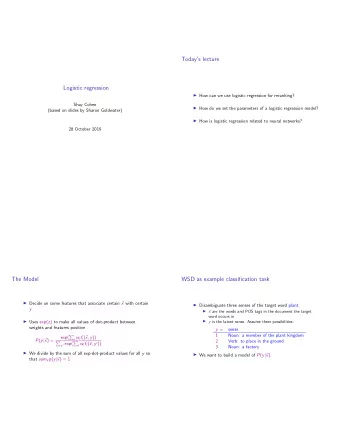
Machine Learning - MT 2016 8. Classification: Logistic Regression Varun Kanade University of Oxford November 2, 2016

Logistic Regression Logistic Regression is actually a classification method In its simplest form it is a binary (two classes) classification method ◮ Today’s Lecture: We’ll denote these by 0 and 1 ◮ Next Week: Sometimes it’s more convenient to call them − 1 and +1 ◮ Ultimately, the choice is just for mathematical convenience It is a discriminative method. We only model: p ( y | w , x ) 1

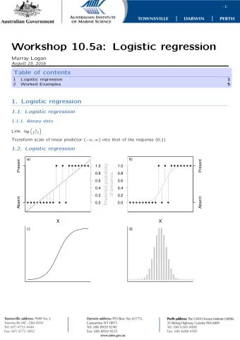
Logistic Regression (LR) ◮ LR builds up on a linear model, composed with a sigmoid function p ( y | w , x ) = Bernoulli(sigmoid( w · x )) ◮ Z ∼ Bernoulli( θ ) � 1 with probability θ Z = 0 with probability 1 − θ ◮ Recall that the sigmoid function is defined by: 1 sigmoid( t ) = 1 + e − t 1 Sigmoid 0 . 8 0 . 6 0 . 4 0 . 2 0 − 4 − 2 0 2 4 t ◮ As we did in the case of linear models, we assume x 0 = 1 for all datapoints, so we do not need to handle the bias term w 0 separately 2

Prediction Using Logistic Regression Suppose we have estimated the model parameters w ∈ R D For a new datapoint x new , the model gives us the probability 1 p ( y new = 1 | x new , w ) = sigmoid( w · x new ) = 1 + exp( − x new · w ) In order to make a prediction we can simply use a threshold at 1 2 y new = I (sigmoid( w · x new )) ≥ 1 � 2) = I ( w · x new ≥ 0) Class boundary is linear (separating hyperplane) 3

Prediction Using Logistic Regression 4

Likelihood of Logistic Regression i =1 , where x i ∈ R D and y i ∈ { 0 , 1 } Data D = � ( x i , y i ) � N Let us denote the sigmoid function by σ We can write the likelihood for of observing the data given model parameters w as: � N σ ( w T x i ) y i · (1 − σ ( w T x i )) 1 − y i p ( y | X , w ) = i =1 Let us denote µ i = σ ( w T x i ) We can write the negative log-likelihood as: N � NLL( y | X , w ) = − ( y i log µ i + (1 − y i ) log(1 − µ i )) i =1 5

Likelihood of Logistic Regression Recall that µ i = σ ( w T x i ) and the negative log-likelihood is N � NLL( y | X , w ) = − ( y i log µ i + (1 − y i ) log(1 − µ i )) i =1 Let us focus on a single datapoint, the contribution to the negative log-likelihood is NLL( y i | x i , w ) = − ( y i log µ i + (1 − y i ) log(1 − µ i )) This is basically the cross-entropy between y i and µ i If y i = 1 , then as ◮ As µ i → 1 , NLL( y i | x i , w ) → 0 ◮ As µ i → 0 , NLL( y i | x i , w ) → ∞ 6

Maximum Likelihood Estimate for LR Recall that µ i = σ ( w T x i ) and the negative log-likelihood is N � NLL( y | X , w ) = − ( y i log µ i + (1 − y i ) log(1 − µ i )) i =1 We can take the gradient with respect to w N � x i ( µ i − y i ) = X T ( µ − y ) ∇ w NLL( y | X , w ) = i =1 And the Hessian is given by, H = X T SX S is a diagonal matrix where S ii = µ i (1 − µ i ) 7

Iteratively Re-Weighted Least Squares (IRLS) Depending on the dimension, we can apply Newton’s method to estimate w Let w t be the parameters after t Newton steps. The gradient and Hessian are given by: g t = X T ( µ t − y ) = − X T ( y − µ t ) H t = X T S t X The Newton Update Rule is: w t +1 = w t − H − 1 t g t = w t + ( X T S t X ) − 1 X T ( y − µ t ) = ( X T S t X ) − 1 X T S t ( Xw t + S − 1 t ( y − µ t )) = ( X T S t X ) − 1 X T S t z t Where z t = Xw t + S − 1 t ( y − µ t ) . Then w t +1 is a solution of the following: Weighted Least Squares Problem N � S t,ii ( z t,i − w T x i ) 2 minimise i =1 8

Multiclass Logistic Regression Multiclass logistic regression is also a discriminative classifier Let the inputs be x ∈ R D and y ∈ { 1 , . . . , C } There are parameters w c ∈ R D for every class c = 1 , . . . , C We’ll put this together in a matrix form W that is D × C The multiclass logistic model is given by: exp( w T c x ) p ( y = c | x , W ) = � C c ′ =1 exp( w T c ′ x ) 9

Multiclass Logistic Regression The multiclass logistic model is given by: exp( w T c x ) p ( y = c | x , W ) = � C c ′ =1 exp( w T c ′ x ) Recall the softmax function Softmax Softmax maps a set of numbers to a probability distribution with mode at the maximum � e a 1 � T � [ a 1 , . . . , a C ] T � Z , . . . , e a C softmax = Z C � e a c . where Z = c =1 The multiclass logistic model is simply: �� � T � w T 1 x , . . . , w T p ( y | x , W ) = softmax C x 10

Multiclass Logistic Regression 11

Summary: Logistic Regression ◮ Logistic Regression is a (binary) classification method ◮ It is a discriminative model ◮ Extension to multiclass by replacing sigmoid by softmax ◮ Can derive Maximum Likelihood Estimates using Convex Optimization ◮ See Chap 8.3 in Murphy (for multiclass), but we’ll revisit as a form of a neural network 12

Next Week ◮ Suppor Vector Machines ◮ Kernel Methods ◮ Revise Linear Programming and Convex Optimisation 13