Introduction to Machine Learning Classification: Logistic Regression - PowerPoint PPT Presentation

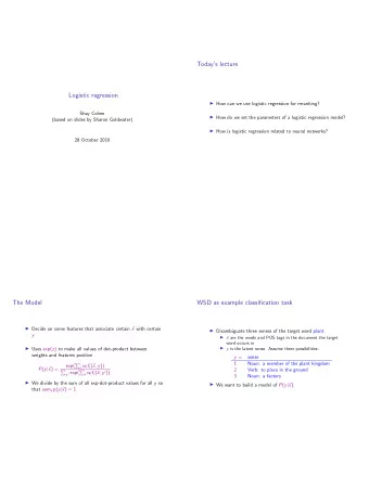
Introduction to Machine Learning Classification: Logistic Regression compstat-lmu.github.io/lecture_i2ml

MOTIVATION A discriminant approach for directly modeling the posterior probabilities π ( x | θ ) of the labels is logistic regression . For now, let’s focus on the binary case y ∈ { 0 , 1 } and use empirical risk minimization. n � � x ( i ) | θ �� � y ( i ) , π arg min R emp ( θ ) = arg min L . θ ∈ Θ θ ∈ Θ i = 1 A naive approach would be to model π ( x | θ ) = θ T x . NB: We will often suppress the intercept in notation. Obviously this could result in predicted probabilities π ( x | θ ) �∈ [ 0 , 1 ] . � c Introduction to Machine Learning – 1 / 8

LOGISTIC FUNCTION To avoid this, logistic regression “squashes” the estimated linear scores θ T x to [ 0 , 1 ] through the logistic function s : θ T x � � exp 1 θ T x � � π ( x | θ ) = 1 + exp ( θ T x ) = 1 + exp ( − θ T x ) = s 1.00 0.75 s(f) 0.50 0.25 0.00 −10 −5 0 5 10 f � c Introduction to Machine Learning – 2 / 8

LOGISTIC FUNCTION exp( θ 0 + f ) The intercept shifts s ( f ) horizontally s ( θ 0 + f ) = 1 +exp( θ 0 + f ) 1.00 θ 0 0.75 −3 0.50 s 0 3 0.25 0.00 −10 −5 0 5 10 f exp( α f ) Scaling f like s ( α f ) = 1 +exp( α f ) : controls the slope and direction. 1.00 α 0.75 −2 −0.3 0.50 s 1 0.25 6 0.00 −10 −5 0 5 10 f � c Introduction to Machine Learning – 3 / 8

BERNOULLI / LOG LOSS We need to define a loss function for the ERM approach: L ( y , π ( x )) = − y ln( π ( x )) − ( 1 − y ) ln( 1 − π ( x )) Penalizes confidently wrong predictions heavily Called Bernoulli, log or cross-entropy loss We can derive it from the negative log-likelihood of Bernoulli / Logistic regression model in statistics Used for many other classifiers, e.g., in NNs or boosting 6 L ( y , π ( x )) y 4 0 1 2 0 0.00 0.25 0.50 0.75 1.00 π ( x ) � c Introduction to Machine Learning – 4 / 8

LOGISTIC REGRESSION IN 1D With one feature x ∈ R . The figure shows data and x �→ π ( x ) . 1.00 ● ● ● ● ● 0.75 ● ● ● ● π ( x ) 0.50 ● ● 0.25 ● ● ● ● 0.00 ● ● ● ● ● 0 2 4 6 x � c Introduction to Machine Learning – 5 / 8

LOGISTIC REGRESSION IN 2D Obviously, logistic regression is a linear classifier, as θ T x � � π ( x | θ ) = s and s is isotonic. logreg: model=FALSE Train: mmce=0.075; CV: mmce.test.mean=0.125 6 ● ● ● ● y 4 ● x2 ● FALSE ● ● TRUE ● ●● ● ● ● ● ● ● 2 ● ● ● ● ● ● 0 0 2 4 6 x1 � c Introduction to Machine Learning – 6 / 8

LOGISTIC REGRESSION IN 2D 1.00 ● ● ● ● ● ● ● ● ● ● ● ● ● ● ● 0.75 ● prob ● 0.50 ● ● ● 0.25 ● ● ● ● ● ● ● ● 0.00 ● ● ● ● ● ● ● ● ● −10 −5 0 5 10 score � c Introduction to Machine Learning – 7 / 8

SUMMARY Hypothesis Space: π : X → [ 0 , 1 ] | π ( x ) = s ( θ T x ) � � H = Risk: Logistic/Bernoulli loss function. L ( y , π ( x )) = − y ln( π ( x )) − ( 1 − y ) ln( 1 − π ( x )) Optimization: Numerical optimization, typically gradient based methods. � c Introduction to Machine Learning – 8 / 8