Lecture 2: Linear Classification Princeton University COS 495 - PowerPoint PPT Presentation

Machine Learning Basics Lecture 2: Linear Classification Princeton University COS 495 Instructor: Yingyu Liang

Review: machine learning basics

Math formulation • Given training data 𝑦 𝑗 , 𝑧 𝑗 : 1 ≤ 𝑗 ≤ 𝑜 i.i.d. from distribution 𝐸 1 • Find 𝑧 = 𝑔(𝑦) ∈ 𝓘 that minimizes ෠ 𝑜 𝑜 σ 𝑗=1 𝑀 𝑔 = 𝑚(𝑔, 𝑦 𝑗 , 𝑧 𝑗 ) • s.t. the expected loss is small 𝑀 𝑔 = 𝔽 𝑦,𝑧 ~𝐸 [𝑚(𝑔, 𝑦, 𝑧)]

Machine learning 1-2-3 • Collect data and extract features • Build model: choose hypothesis class 𝓘 and loss function 𝑚 • Optimization: minimize the empirical loss

Machine learning 1-2-3 Experience • Collect data and extract features • Build model: choose hypothesis class 𝓘 and loss function 𝑚 • Optimization: minimize the empirical loss Prior knowledge

Example: Linear regression • Given training data 𝑦 𝑗 , 𝑧 𝑗 : 1 ≤ 𝑗 ≤ 𝑜 i.i.d. from distribution 𝐸 1 𝑥 𝑦 = 𝑥 𝑈 𝑦 that minimizes ෠ 𝑜 𝑥 𝑈 𝑦 𝑗 − 𝑧 𝑗 2 • Find 𝑔 𝑜 σ 𝑗=1 𝑀 𝑔 𝑥 = 𝑚 2 loss Linear model 𝓘

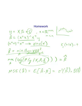
Why 𝑚 2 loss • Why not choose another loss • 𝑚 1 loss, hinge loss, exponential loss, … • Empirical: easy to optimize • For linear case: w = 𝑌 𝑈 𝑌 −1 𝑌 𝑈 𝑧 • Theoretical: a way to encode prior knowledge Questions: • What kind of prior knowledge? • Principal way to derive loss?

Maximum likelihood Estimation

Maximum likelihood Estimation (MLE) • Given training data 𝑦 𝑗 , 𝑧 𝑗 : 1 ≤ 𝑗 ≤ 𝑜 i.i.d. from distribution 𝐸 • Let {𝑄 𝜄 𝑦, 𝑧 : 𝜄 ∈ Θ} be a family of distributions indexed by 𝜄 • Would like to pick 𝜄 so that 𝑄 𝜄 (𝑦, 𝑧) fits the data well

Maximum likelihood Estimation (MLE) • Given training data 𝑦 𝑗 , 𝑧 𝑗 : 1 ≤ 𝑗 ≤ 𝑜 i.i.d. from distribution 𝐸 • Let {𝑄 𝜄 𝑦, 𝑧 : 𝜄 ∈ Θ} be a family of distributions indexed by 𝜄 • “fitness” of 𝜄 to one data point 𝑦 𝑗 , 𝑧 𝑗 likelihood 𝜄; 𝑦 𝑗 , 𝑧 𝑗 ≔ 𝑄 𝜄 (𝑦 𝑗 , 𝑧 𝑗 )

Maximum likelihood Estimation (MLE) • Given training data 𝑦 𝑗 , 𝑧 𝑗 : 1 ≤ 𝑗 ≤ 𝑜 i.i.d. from distribution 𝐸 • Let {𝑄 𝜄 𝑦, 𝑧 : 𝜄 ∈ Θ} be a family of distributions indexed by 𝜄 • “fitness” of 𝜄 to i.i.d. data points { 𝑦 𝑗 , 𝑧 𝑗 } ≔ 𝑄 𝜄 {𝑦 𝑗 , 𝑧 𝑗 } = ς 𝑗 𝑄 𝜄 (𝑦 𝑗 , 𝑧 𝑗 ) likelihood 𝜄; {𝑦 𝑗 , 𝑧 𝑗 }

Maximum likelihood Estimation (MLE) • Given training data 𝑦 𝑗 , 𝑧 𝑗 : 1 ≤ 𝑗 ≤ 𝑜 i.i.d. from distribution 𝐸 • Let {𝑄 𝜄 𝑦, 𝑧 : 𝜄 ∈ Θ} be a family of distributions indexed by 𝜄 • MLE: maximize “fitness” of 𝜄 to i.i.d. data points { 𝑦 𝑗 , 𝑧 𝑗 } 𝜄 𝑁𝑀 = argmax θ∈Θ ς 𝑗 𝑄 𝜄 (𝑦 𝑗 , 𝑧 𝑗 )

Maximum likelihood Estimation (MLE) • Given training data 𝑦 𝑗 , 𝑧 𝑗 : 1 ≤ 𝑗 ≤ 𝑜 i.i.d. from distribution 𝐸 • Let {𝑄 𝜄 𝑦, 𝑧 : 𝜄 ∈ Θ} be a family of distributions indexed by 𝜄 • MLE: maximize “fitness” of 𝜄 to i.i.d. data points { 𝑦 𝑗 , 𝑧 𝑗 } 𝜄 𝑁𝑀 = argmax θ∈Θ log[ς 𝑗 𝑄 𝜄 𝑦 𝑗 , 𝑧 𝑗 ] 𝜄 𝑁𝑀 = argmax θ∈Θ σ 𝑗 log[𝑄 𝜄 𝑦 𝑗 , 𝑧 𝑗 ]

Maximum likelihood Estimation (MLE) • Given training data 𝑦 𝑗 , 𝑧 𝑗 : 1 ≤ 𝑗 ≤ 𝑜 i.i.d. from distribution 𝐸 • Let {𝑄 𝜄 𝑦, 𝑧 : 𝜄 ∈ Θ} be a family of distributions indexed by 𝜄 • MLE: negative log-likelihood loss 𝜄 𝑁𝑀 = argmax θ∈Θ σ 𝑗 log(𝑄 𝜄 𝑦 𝑗 , 𝑧 𝑗 ) 𝑚 𝑄 𝜄 , 𝑦 𝑗 , 𝑧 𝑗 = − log(𝑄 𝜄 𝑦 𝑗 , 𝑧 𝑗 ) ෠ 𝑀 𝑄 𝜄 = − σ 𝑗 log(𝑄 𝜄 𝑦 𝑗 , 𝑧 𝑗 )

MLE: conditional log-likelihood • Given training data 𝑦 𝑗 , 𝑧 𝑗 : 1 ≤ 𝑗 ≤ 𝑜 i.i.d. from distribution 𝐸 • Let {𝑄 𝜄 𝑧 𝑦 : 𝜄 ∈ Θ} be a family of distributions indexed by 𝜄 Only care about predicting y • MLE: negative conditional log-likelihood loss from x; do not care about p(x) 𝜄 𝑁𝑀 = argmax θ∈Θ σ 𝑗 log(𝑄 𝜄 𝑧 𝑗 |𝑦 𝑗 ) 𝑚 𝑄 𝜄 , 𝑦 𝑗 , 𝑧 𝑗 = − log(𝑄 𝜄 𝑧 𝑗 |𝑦 𝑗 ) ෠ 𝑀 𝑄 𝜄 = − σ 𝑗 log(𝑄 𝜄 𝑧 𝑗 |𝑦 𝑗 )

MLE: conditional log-likelihood • Given training data 𝑦 𝑗 , 𝑧 𝑗 : 1 ≤ 𝑗 ≤ 𝑜 i.i.d. from distribution 𝐸 • Let {𝑄 𝜄 𝑧 𝑦 : 𝜄 ∈ Θ} be a family of distributions indexed by 𝜄 P(y|x): discriminative; • MLE: negative conditional log-likelihood loss P(x,y): generative 𝜄 𝑁𝑀 = argmax θ∈Θ σ 𝑗 log(𝑄 𝜄 𝑧 𝑗 |𝑦 𝑗 ) 𝑚 𝑄 𝜄 , 𝑦 𝑗 , 𝑧 𝑗 = − log(𝑄 𝜄 𝑧 𝑗 |𝑦 𝑗 ) ෠ 𝑀 𝑄 𝜄 = − σ 𝑗 log(𝑄 𝜄 𝑧 𝑗 |𝑦 𝑗 )

Example: 𝑚 2 loss • Given training data 𝑦 𝑗 , 𝑧 𝑗 : 1 ≤ 𝑗 ≤ 𝑜 i.i.d. from distribution 𝐸 1 𝜄 𝑦 that minimizes ෠ 𝑜 𝜄 (𝑦 𝑗 ) − 𝑧 𝑗 2 • Find 𝑔 𝑜 σ 𝑗=1 𝑀 𝑔 𝜄 = 𝑔

Example: 𝑚 2 loss • Given training data 𝑦 𝑗 , 𝑧 𝑗 : 1 ≤ 𝑗 ≤ 𝑜 i.i.d. from distribution 𝐸 1 𝜄 𝑦 that minimizes ෠ 𝑜 𝜄 (𝑦 𝑗 ) − 𝑧 𝑗 2 • Find 𝑔 𝑜 σ 𝑗=1 𝑀 𝑔 𝜄 = 𝑔 𝑚 2 loss: Normal + MLE • Define 𝑄 𝜄 𝑧 𝑦 = Normal 𝑧; 𝑔 𝜄 𝑦 , 𝜏 2 −1 1 − 𝑧 𝑗 ) 2 −log(𝜏) − • log(𝑄 𝜄 𝑧 𝑗 |𝑦 𝑗 ) = 2𝜏 2 (𝑔 𝜄 𝑦 𝑗 2 log(2𝜌) 1 𝑜 𝜄 (𝑦 𝑗 ) − 𝑧 𝑗 2 • 𝜄 𝑁𝑀 = argmin θ∈Θ 𝑜 σ 𝑗=1 𝑔

Linear classification

Example 1: image classification indoor Indoor outdoor

Example 2: Spam detection #”$” #”Mr.” #”sale” … Spam? Email 1 2 1 1 Yes Email 2 0 1 0 No Email 3 1 1 1 Yes … Email n 0 0 0 No New email 0 0 1 ??

Why classification • Classification: a kind of summary • Easy to interpret • Easy for making decisions

Linear classification 𝑥 𝑈 𝑦 = 0 𝑥 𝑈 𝑦 > 0 𝑥 𝑈 𝑦 < 0 𝑥 Class 1 Class 0

Linear classification: natural attempt • Given training data 𝑦 𝑗 , 𝑧 𝑗 : 1 ≤ 𝑗 ≤ 𝑜 i.i.d. from distribution 𝐸 𝑥 𝑦 = 𝑥 𝑈 𝑦 • Hypothesis 𝑔 • 𝑧 = 1 if 𝑥 𝑈 𝑦 > 0 Linear model 𝓘 • 𝑧 = 0 if 𝑥 𝑈 𝑦 < 0 𝑥 𝑦 ) = step(𝑥 𝑈 𝑦) • Prediction: 𝑧 = step(𝑔

Linear classification: natural attempt • Given training data 𝑦 𝑗 , 𝑧 𝑗 : 1 ≤ 𝑗 ≤ 𝑜 i.i.d. from distribution 𝐸 1 𝑥 𝑦 = 𝑥 𝑈 𝑦 to minimize ෠ 𝑜 𝕁[step(𝑥 𝑈 𝑦 𝑗 ) ≠ 𝑧 𝑗 ] • Find 𝑔 𝑜 σ 𝑗=1 𝑀 𝑔 𝑥 = • Drawback: difficult to optimize • NP-hard in the worst case 0-1 loss

Linear classification: simple approach • Given training data 𝑦 𝑗 , 𝑧 𝑗 : 1 ≤ 𝑗 ≤ 𝑜 i.i.d. from distribution 𝐸 1 𝑥 𝑦 = 𝑥 𝑈 𝑦 that minimizes ෠ 𝑜 𝑥 𝑈 𝑦 𝑗 − 𝑧 𝑗 2 • Find 𝑔 𝑜 σ 𝑗=1 𝑀 𝑔 𝑥 = Reduce to linear regression; ignore the fact 𝑧 ∈ {0,1}

Linear classification: simple approach Drawback: not robust to “outliers” Figure borrowed from Pattern Recognition and Machine Learning , Bishop

Compare the two 𝑧 𝑧 = 𝑥 𝑈 𝑦 𝑧 = step(𝑥 𝑈 𝑦) 𝑥 𝑈 𝑦

Between the two • Prediction bounded in [0,1] • Smooth 1 • Sigmoid: 𝜏 𝑏 = 1+exp(−𝑏) Figure borrowed from Pattern Recognition and Machine Learning , Bishop

Linear classification: sigmoid prediction • Squash the output of the linear function 1 Sigmoid 𝑥 𝑈 𝑦 = 𝜏 𝑥 𝑈 𝑦 = 1 + exp(−𝑥 𝑈 𝑦) 1 • Find 𝑥 that minimizes ෠ 𝑜 𝜏(𝑥 𝑈 𝑦 𝑗 ) − 𝑧 𝑗 2 𝑜 σ 𝑗=1 𝑀 𝑔 𝑥 =

Linear classification: logistic regression • Squash the output of the linear function 1 Sigmoid 𝑥 𝑈 𝑦 = 𝜏 𝑥 𝑈 𝑦 = 1 + exp(−𝑥 𝑈 𝑦) • A better approach: Interpret as a probability 1 𝑥 (𝑧 = 1|𝑦) = 𝜏 𝑥 𝑈 𝑦 = 𝑄 1 + exp(−𝑥 𝑈 𝑦) 𝑥 𝑧 = 1 𝑦 = 1 − 𝜏 𝑥 𝑈 𝑦 𝑄 𝑥 𝑧 = 0 𝑦 = 1 − 𝑄

Linear classification: logistic regression • Given training data 𝑦 𝑗 , 𝑧 𝑗 : 1 ≤ 𝑗 ≤ 𝑜 i.i.d. from distribution 𝐸 • Find 𝑥 that minimizes 𝑜 𝑀 𝑥 = − 1 ෠ 𝑜 ෍ log 𝑄 𝑥 𝑧 𝑦 𝑗=1 𝑀 𝑥 = − 1 log𝜏(𝑥 𝑈 𝑦 𝑗 ) − 1 ෠ log[1 − 𝜏 𝑥 𝑈 𝑦 𝑗 ] 𝑜 ෍ 𝑜 ෍ 𝑧 𝑗 =1 𝑧 𝑗 =0 Logistic regression: MLE with sigmoid

Linear classification: logistic regression • Given training data 𝑦 𝑗 , 𝑧 𝑗 : 1 ≤ 𝑗 ≤ 𝑜 i.i.d. from distribution 𝐸 • Find 𝑥 that minimizes 𝑀 𝑥 = − 1 log𝜏(𝑥 𝑈 𝑦 𝑗 ) − 1 ෠ log[1 − 𝜏 𝑥 𝑈 𝑦 𝑗 ] 𝑜 ෍ 𝑜 ෍ 𝑧 𝑗 =1 𝑧 𝑗 =0 No close form solution; Need to use gradient descent