Learning From Data Lecture 8 Linear Classification and Regression - PowerPoint PPT Presentation

Learning From Data Lecture 8 Linear Classification and Regression Linear Classification Linear Regression M. Magdon-Ismail CSCI 4100/6100

recap: Approximation Versus Generalization VC Analysis Bias-Variance Analysis E out ≤ E in + Ω( d vc ) E out = bias + var 1. Did you fit your data well enough ( E in )? 1. How well can you fit your data ( bias )? 2. Are you confident your E in will generalize to E out 2. How close to that best fit can you get ( var )? out-of-sample error y y model complexity Error x x in-sample error d ∗ VC dimension, d vc ¯ g ( x ) vc y y g ( x ) ¯ sin( x ) sin( x ) x x The VC Insuarance Co. H 0 H 1 The VC warranty had conditions for becoming void: bias = 0 . 50; bias = 0 . 21; var = 0 . 25. var = 1 . 69. You can’t look at your data before choosing H . E out = 0 . 75 � E out = 1 . 90 Data must be generated i.i.d from P ( x ). Data and test case from same P ( x ) (same bin). M Linear Classification and Regression : 2 /23 � A c L Creator: Malik Magdon-Ismail Recap: learning curve − →

recap: Decomposing The Learning Curve VC Analysis Bias-Variance Analysis Expected Error Expected Error E out E out variance generalization error E in E in bias in-sample error Number of Data Points, N Number of Data Points, N Pick H that can generalize and has a good Pick ( H , A ) to approximate f and not behave chance to fit the data wildly after seeing the data M Linear Classification and Regression : 3 /23 � A c L Creator: Malik Magdon-Ismail 3 learning problems − →

Three Learning Problems Approve Classification y = ± 1 or Deny Credit Amount y ∈ R Regression Analysis of Credit Probability y ∈ [0 , 1] Logistic Regression of Default • Linear models are perhaps the fundamental model. • The linear model is the first model to try. M Linear Classification and Regression : 4 /23 � A c L Creator: Malik Magdon-Ismail Linear signal − →

The Linear Signal linear in x : gives the line/hyperplane separator ↓ s = w t x ↑ linear in w : makes the algorithms work x is the augmented vector: x ∈ { 1 } × R d M Linear Classification and Regression : 5 /23 � A c L Creator: Malik Magdon-Ismail Using the linear signal − →

The Linear Signal   → sign( w t x )  {− 1 , +1 }              → w t x s = w t x − → R            → θ ( w t x )  [0 , 1]    y = θ ( s ) M Linear Classification and Regression : 6 /23 � A c L Creator: Malik Magdon-Ismail Classification and PLA − →

Linear Classification � h ( x ) = sign( w t x ) � H lin = 1. E in ≈ E out because d vc = d + 1, �� � d E out ( h ) ≤ E in ( h ) + O N log N . 2. If the data is linearly separable, PLA will find a separator = ⇒ E in = 0. w ( t + 1) = w ( t ) + x ∗ y ∗ ↑ misclassified data point E in = 0 = ⇒ E out ≈ 0 ( f is well approximated by a linear fit). What if the data is not separable ( E in = 0 is not possible)? pocket algorithm How to ensure E in ≈ 0 is possible? select good features M Linear Classification and Regression : 7 /23 � A c L Creator: Malik Magdon-Ismail Non-separable data − →

Non-Separable Data M Linear Classification and Regression : 8 /23 � A c L Creator: Malik Magdon-Ismail Pocket algorithm − →

The Pocket Algorithm Minimizing E in is a hard combinatorial problem. The Pocket Algorithm – Run PLA – At each step keep the best E in (and w ) so far. (Its not rocket science, but it works.) (Other approaches: linear regression, logistic regression, linear programming . . . ) M Linear Classification and Regression : 9 /23 � A c L Creator: Malik Magdon-Ismail Digits − →

Digits Data Each digit is a 16 × 16 image. M Linear Classification and Regression : 10 /23 � A c L Creator: Malik Magdon-Ismail Input is 256 dimensional − →

Digits Data Each digit is a 16 × 16 image. � -1 -1 -1 -1 -1 -1 -1 -0.63 0.86 -0.17 -1 -1 -1 -1 -1 -1 -1 -1 -1 -1 -1 -1 -0.99 0.3 1 0.31 -1 -1 -1 -1 -1 -1 -1 -1 -1 -1 -1 -1 -0.41 1 0.99 -0.57 -1 -1 -1 -1 -1 -1 -1 -1 -1 -1 -1 -0.68 0.83 1 0.56 -1 -1 -1 -1 -1 -1 -1 -1 -1 -1 -1 -0.94 0.54 1 0.78 -0.72 -1 -1 -1 -1 -1 -1 -1 -1 -1 -1 -1 0.1 1 0.92 -0.44 -1 -1 -1 -1 -1 -1 -1 -1 -1 -1 -1 -0.26 0.95 1 -0.16 -1 -1 -1 -0.99 -0.71 -0.83 -1 -1 -1 -1 -1 -0.8 0.91 1 0.3 -0.96 -1 -1 -0.55 0.49 1 0.88 0.09 -1 -1 -1 -1 0.28 1 0.88 -0.8 -1 -0.9 0.14 0.97 1 1 1 0.99 -0.74 -1 -1 -0.95 0.84 1 0.32 -1 -1 0.35 1 0.65 -0.10 -0.18 1 0.98 -0.72 -1 -1 -0.63 1 1 0.07 -0.92 0.11 0.96 0.30 -0.88 -1 -0.07 1 0.64 -0.99 -1 -1 -0.67 1 1 0.75 0.34 1 0.70 -0.94 -1 -1 0.54 1 0.02 -1 -1 -1 -0.90 0.79 1 1 1 1 0.53 0.18 0.81 0.83 0.97 0.86 -0.63 -1 -1 -1 -1 -0.45 0.82 1 1 1 1 1 1 1 1 0.13 -1 -1 -1 -1 -1 � -1 -0.48 0.81 1 1 1 1 1 1 0.21 -0.94 -1 -1 -1 -1 -1 -1 -1 -0.97 -0.42 0.30 0.82 1 0.48 -0.47 -0.99 -1 -1 -1 -1 � x = (1 , x 1 , · · · , x 256 ) ← input d vc = 257 w = ( w 0 , w 1 , · · · , w 256 ) ← linear model M Linear Classification and Regression : 11 /23 � A c L Creator: Malik Magdon-Ismail Intensity and symmetry features − →

Intensity and Symmetry Features feature : an important property of the input that you think is useful for classification. ( dictionary.com : a prominent or conspicuous part or characteristic) � x = (1 , x 1 , x 2 ) ← input d vc = 3 w = ( w 0 , w 1 , w 2 ) ← linear model M Linear Classification and Regression : 12 /23 � A c L Creator: Malik Magdon-Ismail PLA on digits data − →

PLA on Digits Data PLA 50% E out Error (log scale) 10% 1% E in 0 250 500 750 1000 Iteration Number, t M Linear Classification and Regression : 13 /23 � A c L Creator: Malik Magdon-Ismail Pocket on digits data − →

Pocket on Digits Data PLA Pocket 50% 50% E out Error (log scale) Error (log scale) 10% 10% E out 1% 1% E in E in 0 250 500 750 1000 0 250 500 750 1000 Iteration Number, t Iteration Number, t M Linear Classification and Regression : 14 /23 � A c L Creator: Malik Magdon-Ismail Regression − →

Linear Regression age 32 years gender male salary 40,000 debt 26,000 years in job 1 year years at home 3 years . . . . . . Classification: Approve/Deny Regression: Credit Line (dollar amount) regression ≡ y ∈ R d � h ( x ) = w i x i = w t x i =0 M Linear Classification and Regression : 15 /23 � A c L Creator: Malik Magdon-Ismail Regression − →

Linear Regression age 32 years gender male salary 40,000 debt 26,000 years in job 1 year years at home 3 years . . . . . . Classification: Approve/Deny Regression: Credit Line (dollar amount) regression ≡ y ∈ R d � w i x i = w t x h ( x ) = i =0 M Linear Classification and Regression : 16 /23 � A c L Creator: Malik Magdon-Ismail Squared error − →

Least Squares Linear Regression y y x 1 x 2 x M Linear Classification and Regression : 17 /23 � A c L Creator: Malik Magdon-Ismail Squared error − →

Least Squares Linear Regression y y x 1 x 2 x y = f ( x ) + ǫ ← − noisy target P ( y | x )  N  � E in ( h ) = 1 ( h ( x n ) − y n ) 2  in-sample error   N n =1 h ( x ) = w t x    E out ( h ) = E x [( h ( x ) − y ) 2 ] out-of-sample error  M Linear Classification and Regression : 18 /23 � A c L Creator: Malik Magdon-Ismail Matrix representation − →

Using Matrices for Linear Regression         — x 1 — ˆ w t x 1 y 1 y 1 — x 2 — ˆ w t x 2 y 2 y 2         ˆ X = y = y =  =  = X w  .   .   .   .  . . . . . . . .       — x N — ˆ w t x N y N y N � �� � � �� � � �� � target vector in-sample predictions data matrix, N × ( d + 1) N E in ( w ) = 1 � y n − y n ) 2 (ˆ N n =1 | 2 1 = N | | ˆ y − y | 2 | 2 1 = N | | X w − y | 2 1 = N ( w t X t X w − 2 w t X t y + y t y ) M Linear Classification and Regression : 19 /23 � A c L Creator: Malik Magdon-Ismail Pseudoinverse solution − →

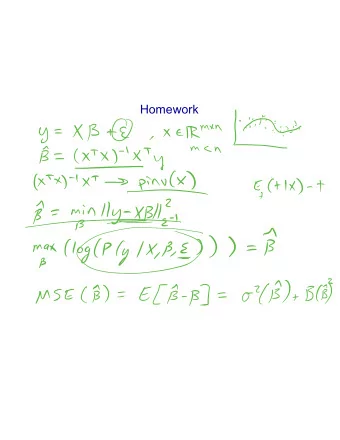
Linear Regression Solution E in ( w ) = 1 N ( w t X t X w − 2 w t X t y + y t y ) Vector Calculus: To minimize E in ( w ), set ∇ w E in ( w ) = 0 . ∇ w ( w t A w ) = (A + A t ) w , ∇ w ( w t b ) = b . A = X t X and b = X t y : ∇ w E in ( w ) = 2 N (X t X w − X t y ) Setting ∇ E in ( w ) = 0 : X t X w = X t y ← − normal equations w lin = (X t X) − 1 X t y ← − when X t X is invertible M Linear Classification and Regression : 20 /23 � A c L Creator: Malik Magdon-Ismail Regression algorithm − →

Linear Regression Algorithm Linear Regression Algorithm: 1. Construct the matrix X and the vector y from the data set ( x 1 , y 1 ) , · · · , ( x N , y N ), where each x includes the x 0 = 1 coordinate,     — x 1 — y 1 — x 2 — y 2     X = y = , .  .   .  . . . .     — x N — y N � �� � � �� � target vector data matrix 2. Compute the pseudo inverse X † of the matrix X. If X t X is invertible, X † = (X t X) − 1 X t 3. Return w lin = X † y . M Linear Classification and Regression : 21 /23 � A c L Creator: Malik Magdon-Ismail Generalization − →