1D Regression i.i.d. with mean 0. Univariate Linear - PDF document
1D Regression i.i.d. with mean 0. Univariate Linear Regression: fit by least squares. Minimize:
✏ ✌ ✁ ✑ ✏ ✏ ✏ ✌ ✠ ☛ ✁ � 1D Regression ☛ ✂☎✄✝✆✟✞✡✠ ☛ i.i.d. with mean 0. ☛ Univariate Linear Regression: ✂☎✄✝✆✟✞☞✁ ✍✎✆ fit by least squares. Minimize: ✄✝� ✂✓✄✔✆ ✞✕✞✕✖ ✄✝� ✍✗✆ ✞✘✖ ✏✒✑ ✏✒✑ ✌✚✙✗✍ . to get ☛ The set of all possible functions is ..... – 1 –
Non-linear problems ➠ What if the underlying function is not linear? ➠ Try: fit non-linear function from a bag of functions ➠ Problem: which bag? The space of all functions is HUGE ➠ Another problem: We only have SOME data: want to find the underlying function but avoid noise ➠ Need to be selective in choosing possible non-linear functions – 2 –
✆ ✌ ✙ ✲ ✁ ✠ ✌ ✻ ✩ ✜ ✄ ✻ ✣ ✜ ✮ ✞ ✆ ✭ ✏ ✜ ✙ ✣ ✜ ✰ ✁ ✜ ✰ ✏ ✞ ✹ ✠ ✰ Basis expansion: polynomial terms ➠ Univariate LS has two basis functions: ✛✢✜✤✣ ✜✒✩ ✄✔✆✥✞✦✁ ✧★✙ ✄✝✆✟✞✪✁ ✆✬✫ ✩ : ➠ The resulting fit is a linear combination of ✂☎✄✝✆✟✞☞✁ ✄✝✆✟✞✡✠ ✍✯✮ ✄✔✆✥✞☞✁ ✍☞✮✦✆ ➠ One way: add non-linear functions of to the bag. Polynomial terms seem as good as any: ✜✱✰ ✄✔✆✥✞☞✁ ✳✴✙✶✵✷✵✶✵✸✙✺✹ ➠ Construct matrix , with: ✄✔✆ ✧ terms ➠ and fit linear regression with – 3 –
Global vs Local fits ➠ One problem with polynomial regression: global fit ➠ Must find very good global basis for global fit: unlikely to find the “true” one ➠ Other way: fit locally with “simple” functions ➠ Why it works: It is easier to find a suitable basis for a part of a function. ➠ Tradeoff: in each part we only have a fraction of data to work with: must be extra-careful not to overfit. – 4 –
✼ ✼ ✩ ✰ ❄ ✑ ✛ ✖ ✼ ✖ ✼ ✧ Polynomial Splines ➠ Flebility: fit low-order polynomials in small ✆ . windows of the support of ➠ Most popular are order 4 (cubic) splines ➠ Must join the pieces somehow: with M-order splines we make sure derivatives up-to M-2 order match at knots ➠ “Naive” basis for cubic splines: ✜✤✼ ✄✝✆✟✞☞✁ ✵✽✆ ✙✾✆ ✙✕✆❀✿ but many coefficents constrained by macthing derivatives ➠ Truncated-power basis set: ✰❋❊ ✧❁✙✕✆❂✙✕✆ ✙✕✆❀✿❃✙ ✄✝✆ ✞❅✿ ❆❇✫❉❈ equivalent to “naive” set plus constraints ➠ Procedure: – 5 –
● ✆ ❄ ✰ ✁ ● ✻ ● ✙❍✲ ✧★✙✷✵✶✵✷✵✸✙❏■ choose knots, populate matrix using truncated power basis set (in columns) each evaluated at all ✏ (rows) data points, Run linear regression with ?? terms. ✂✓✄✔✆✥✞ linear beyond data: ➠ Natural Cubic splines: extra two constraints on each side ➠ The number of parameters (degrees of freedom) is now ? – 6 –
❲ ❲ ❚ ✁ ✰ ❩ ❨ ❳ ✖ ✞ ✏ ✰ ✜ ✰ ❚ ✰ ✑ ✏ � ✏ ✆ ❙ Regularization ➠ Avoid knot-selection problem. Use all possible ✏ ’s) knots (unique ➠ But have over-parameterized regression (N+2 parameters, N data points) ➠ Need to regularize (shrink) coeficients: ❑✢▲✾▼❖◆ P❘◗ ✄✝✆ ❙❱❯☎❲❇❙ subject to: ➠ Without constraint we get usual least squares fit: here we get infinite number of them ➠ The constraint on only allows those fits with certain ❚ . controls over-all smoothness of the final fit: ➠ ✰❬❩ ✜❪❭❫❭ ✜✤❭❫❭ ✄✝✆✟✞ ✄✝✆✟✞❵❴❛✆ – 7 –
✛ ❡ ✏ ❤ ❜ ✏ ✆ ✏ ✑ ✖ ✏ ✂ ✖ ✠ ❝ ❞ ➠ This remarkably solves a general variational problem: ❭❫❭ ❑✢▲❏▼❛◆ P❘◗ ✄✝� ✂✓✄✔✆ ✞✕✞ ✄❣❢✾✞✎✫ ❴★❢ ❨ above. ❝ is in one-to-one correspondance with ➠ Solution: Natural Cubic Spline with knots at each ✏ . ✂☎✄✝✆ ✞ in O(N). ➠ Benefit: Can get all fits – 8 –
❲ ✄ ❝ ✠ ✻ ❭ ✻ ✄ ✏ ✻ ✰ ✭q ✁ ✻ ✻ ❲ ✻ ❭ ✻ ✠ ✐ ✄ ❥ ✐ ✠ ❝ ❲ ✩ ✻ ♦ B-spline Basis ☛ Most smoothing splines computationally fitted using B-spline basis ☛ B-spline are a basis for polynomial splines on a closed interval. Each cubic B-spline spans at most 5 knots. ❦❁✞ ☛ Computationally, one sets up an matrix of ordered, evaluated B-spline basis. ✲ , is a ✲ th B-spline, and its center Each column, moves from left-most to right-most point. ✞ , has banded structure and so does ☛ where: ❭❫❭ ❭❫❭ ✄✔❧♠✙❍✲♥✞☞✁ ✄♣❢✾✞❵♦ ✄❣❢❏✞❵❴★❢ ☛ One then solves a penalized regression problem: ❭ts ✞✎r ☛ This is actually done using Choleski and – 9 –
✛ ✭ ✑ s ❝ ❜ ① ① ✁ ✂ ✖ ✖ ❳ ✰ ♦ ✰ ✉ ✰ ❨ ✂ ① q back-substitution to get O(N) running time. ✂ to be fitted is ☛ Conceptually, the function expanded into a B-spline basis set: ✂☎✄✝✆✟✞☞✁ ✄✔✆✥✞ and fit obtained by constrained least-squares: ❑✢▲✾▼❖◆ P❘◗ ✈✇✈ ✈✇✈ subject to penalty: ✄❍✂✟✞ ✄❍✂✟✞ is the familiar squared Here second-derivative functional: ❭❫❭ ✄❍✂✟✞②✁ ✄❣❢✾✞✎✫ ❴★❢ ❨ is one-to-one with and – 10 –
✁ ⑥ ✞ ❯ ✻ ✩ r ✞ ✻ ❯ ✻ ✄ ✻ ✄ ▲ Equivalent DF ➠ Smoothing spline (and many other smoothing procedures) are usually called semi-parametric models ✆ into basis set, it looks like any ➠ Once you expand other regression ✜♥✰ ✄✝✆✟✞ have no real ➠ BUT individual terms, meaning ➠ With penalties, one cannot count number of terms to get degrees of freedom ➠ Equivalent expression is needed for guidance and (approx) inference ➠ In regular regression: ③⑤④ this is the trace of a hat , or projection matrix. ➠ All penalized regressions (including cubic – 11 –
s ✩ ⑥ ⑨ ▲ s ⑨ ✁ ✭ ❯ ⑦ r ❷ ✞ ❲ ❝ ✠ ⑦ ❯ ⑨ ⑦ ✁ s ✁ smoothing splines) are obtained by: ✄⑧⑦ ➠ while is not a projection matrix, it has similar properties (it is a shrunk projection operator) ⑩☞❶ ➠ Define: – 12 –
Recommend
More recommend
Explore More Topics
Stay informed with curated content and fresh updates.
