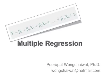
Multiple Linear Regression Often more than one predictor variable - PowerPoint PPT Presentation

ST 370 Probability and Statistics for Engineers Multiple Linear Regression Often more than one predictor variable can be used to predict the value of a response variable. The basic approach of the simple linear regression model may be extended to include multiple predictors. The principles carry over, but the computations are more tedious, and hand calculation is largely infeasible. 1 / 8 Multiple Linear Regression

ST 370 Probability and Statistics for Engineers For example, consider the data on the strength of the bond between a component and its frame: wireBond <- read.csv("Data/Table-01-02.csv") pairs(wireBond) Clearly Length ( x 1 ) could be used to predict Strength ( y ), but also possibly Height ( x 2 ) or Length 2 ( x 2 1 ). 2 / 8 Multiple Linear Regression

ST 370 Probability and Statistics for Engineers Multiple Linear Regression Model The multiple linear regression model with k predictors is Y = β 0 + β 1 x 1 + β 2 x 2 + · · · + β k x k + ǫ Notation When we have n observations on data like these, we write them k � Y i = β 0 + x i , j β j + ǫ i , i = 1 , 2 , . . . , n ; j =1 that is, x i , j is the value of the j th predictor x j in the i th observation. 3 / 8 Multiple Linear Regression Multiple Linear Regression Model

ST 370 Probability and Statistics for Engineers Predictors and Variables Each term in the equation is a predictor , but is not necessarily an independent variable . For example, consider the relationship between Strength and Langth: plot(Strength ~ Length, wireBond) Strength increases with Length, and roughly linearly, so we could use the single-variable equation Y = β 0 + β 1 x + ǫ. 4 / 8 Multiple Linear Regression Multiple Linear Regression Model

ST 370 Probability and Statistics for Engineers Close examination suggests that the relationship may be curved , not linear, so we might want to fit the quadratic equation Y = β 0 + β 1 x + β 2 x 2 + ǫ. If we write x 1 = x , x 2 = x 2 , this becomes Y = β 0 + β 1 x 1 + β 2 x 2 + ǫ, the multiple regression model with k = 2 predictors. But the equation brings in only one independent variable, Length. 5 / 8 Multiple Linear Regression Multiple Linear Regression Model

ST 370 Probability and Statistics for Engineers Least Squares As with the single-predictor model, we usually find parameter estimates using the least squares approach. For any proposed values b 0 , b 1 , . . . , b k we form the predicted values b 0 + b 1 x i , 1 + · · · + b k x i , k , i = 1 , 2 , . . . , n and the residuals e i = y i − ( b 0 + b 1 x i , 1 + · · · + b k x i , k ) , i = 1 , 2 , . . . , n The sum of squares to be minimized is n n � e 2 � [ y i − ( b 0 + b 1 x i , 1 + · · · + b k x i , k )] 2 . L ( b 0 , b 1 , . . . , b k ) = i = i =1 i =1 6 / 8 Multiple Linear Regression Multiple Linear Regression Model

ST 370 Probability and Statistics for Engineers The least squares estimates ˆ β 0 , ˆ β 1 , . . . , ˆ β k that minimize L ( b 0 , b 1 , . . . , b k ) cannot in general be written out in closed form, but have to be found by solving a set of equations. The residual sum of squares is again n � e 2 SS E = i , i =1 but the degrees of freedom for residuals are n − ( k + 1), so the estimate of σ 2 is SS E σ 2 = MS E = ˆ n − ( k + 1) . 7 / 8 Multiple Linear Regression Multiple Linear Regression Model

ST 370 Probability and Statistics for Engineers Fitting the model Use lm() to fit the multiple regression model: # the quadratic model: summary(lm(Strength ~ Length + I(Length^2), wireBond)) # the two-variable model: summary(lm(Strength ~ Length + Height, wireBond)) # quadratic in Strength, plus Height: summary(lm(Strength ~ Length + I(Length^2) + Height, wireBond)) Note The arithmetic operators “ + ”, “ - ”, “ * ”, “ / ”, and “ ^ ” have special meanings within a formula, so the predictor Length^2 must be “wrapped” in the identity function I() , otherwise it is misparsed as part of the formula. 8 / 8 Multiple Linear Regression Multiple Linear Regression Model