w o o o o o o o o x o o o o o x o that represents - PowerPoint PPT Presentation
Outline Logistic function Logistic regression IAML: Logistic Regression Learning logistic regression Optimization Charles Sutton and Victor Lavrenko The power of non-linear basis functions School of Informatics
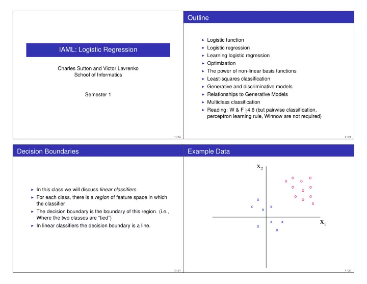
Outline ◮ Logistic function ◮ Logistic regression IAML: Logistic Regression ◮ Learning logistic regression ◮ Optimization Charles Sutton and Victor Lavrenko ◮ The power of non-linear basis functions School of Informatics ◮ Least-squares classification ◮ Generative and discriminative models ◮ Relationships to Generative Models Semester 1 ◮ Multiclass classification ◮ Reading: W & F § 4.6 (but pairwise classification, perceptron learning rule, Winnow are not required) 1 / 24 2 / 24 Decision Boundaries Example Data x 2 o o o o o o ◮ In this class we will discuss linear classifiers . o o o ◮ For each class, there is a region of feature space in which x o o the classifier x x x ◮ The decision boundary is the boundary of this region. (i.e., Where the two classes are “tied”) x 1 x x ◮ In linear classifiers the decision boundary is a line. x x 3 / 24 4 / 24
Linear Classifiers A Geometric View x 2 ◮ In a two-class linear classifier, we o o o o learn a function x 2 o o o F ( x , w ) = w ⊤ x + w 0 w o o o o o o o o x o o o o o x o that represents how aligned the o x x x x x x instance is with y = 1. x 1 x x x x 1 x ◮ w are parameters of the classifier x x x that we learn from data. x ◮ To do prediction of an input x : x �→ ( y = 1 ) if F ( x , w ) > 0 5 / 24 6 / 24 Explanation of Geometric View Two Class Discrimination ◮ For now consider a two class case: y ∈ { 0 , 1 } . ◮ From now on we’ll write x = ( 1 , x 1 , x 2 , . . . x d ) and ◮ The decision boundary in the previous case is w = ( w 0 , w 1 , . . . x d ) . ◮ We will want a linear, probabilistic model. We could try { x | w ⊤ x + w 0 = 0 } P ( y = 1 | x ) = w ⊤ x . But this is stupid. ◮ Instead what we will do is ◮ w is a normal vector to this surface ◮ (Remember how lines can be written in terms of their P ( y = 1 | x ) = f ( w ⊤ x ) normal vector.) ◮ Notice that in more than 2 dimensions, this boundary will ◮ f must be between 0 and 1. It will squash the real line into be a hyperplane. [ 0 , 1 ] ◮ Furthermore the fact that probabilities sum to one means P ( y = 0 | x ) = 1 − f ( w ⊤ x ) 7 / 24 8 / 24
The logistic function Linear weights ◮ We need a function that returns probabilities (i.e. stays between 0 and 1). ◮ Linear weights + logistic squashing function == logistic ◮ The logistic function provides this regression. ◮ f ( z ) = σ ( z ) ≡ 1 / ( 1 + exp ( − z )) . ◮ We model the class probabilities as ◮ As z goes from −∞ to ∞ , so f goes from 0 to 1, a “squashing function” D � w j x j ) = σ ( w T x ) p ( y = 1 | x ) = σ ( ◮ It has a “sigmoid” shape (i.e. S-like shape) j = 0 0.9 ◮ σ ( z ) = 0 . 5 when z = 0. Hence the decision boundary is 0.8 given by w T x + w 0 = 0. 0.7 0.6 ◮ Decision boundary is a M − 1 hyperplane for a M 0.5 0.4 dimensional problem. 0.3 0.2 0.1 − 6 − 4 − 2 0 2 4 6 9 / 24 10 / 24 Logistic regression Learning Logistic Regression ◮ For this slide write ˜ w = ( w 1 , w 2 , . . . w d ) (i.e., exclude the bias w 0 ) ◮ The bias parameter w 0 shifts the position of the ◮ Want to set the parameters w using training data. hyperplane, but does not alter the angle ◮ As before: ◮ The direction of the vector ˜ w affects the angle of the ◮ Write out the model and hence the likelihood hyperplane. The hyperplane is perpendicular to ˜ w ◮ Find the derivatives of the log likelihood w.r.t the ◮ The magnitude of the vector ˜ w effects how certain the parameters. ◮ Adjust the parameters to maximize the log likelihood. classifications are ◮ For small ˜ w most of the probabilities within a region of the decision boundary will be near to 0 . 5. ◮ For large ˜ w probabilities in the same region will be close to 1 or 0. 11 / 24 12 / 24
◮ It turns out that the likelihood has a unique optimum (given ◮ Assume data is independent and identically distributed. sufficient training examples). It is convex . ◮ Call the data set D = { ( x 1 , y 1 ) , ( x 2 , y 2 ) , . . . ( x n , y n ) } ◮ How to maximize? Take gradient ◮ The likelihood is n ∂ L n � ( y i − σ ( w T x i )) x ij = � ∂ w j p ( D | w ) = p ( y = y i | x i , w ) i = 1 i = 1 ◮ (Aside: something similar holds for linear regression n p ( y = 1 | x i , w ) y i ( 1 − p ( y = 1 | x i , w )) 1 − y i � = n ∂ E i = 1 � ( w T φ ( x i ) − y i ) x ij = ∂ w j ◮ Hence the log likelihood L ( w ) = log p ( D | w ) is given by i = 1 where E is squared error.) n � y i log σ ( w ⊤ x i ) + ( 1 − y i ) log ( 1 − σ ( w ⊤ x i )) L ( w ) = ◮ Unfortunately, you cannot maximize L ( w ) explicitly as for i = 1 linear regression. You need to use a numerical method (see next lecture). 13 / 24 14 / 24 Geometric Intuition of Gradient Geometric Intuition of Gradient ◮ One training point, y 1 = 1. ◮ Let’s say there’s only one training point D = { ( x 1 , y 1 ) } . ∂ L = ( y 1 − σ ( w ⊤ x 1 )) x 1 j Then ∂ w j ∂ L = ( y 1 − σ ( w ⊤ x 1 )) x 1 j ◮ Remember: gradient is direction of steepest increase . We ∂ w j want to maximize, so let’s nudge the parameters in the ◮ Also assume y 1 = 1. (It will be symmetric for y 1 = 0.) direction ∂ L ∂ w j ◮ Note that ( y 1 − σ ( w ⊤ x 1 )) is always positive because ◮ If σ ( w ⊤ x 1 ) is correct, e.g., 0 . 99 σ ( z ) < 1 for all z . ◮ Then ( y 1 − σ ( w ⊤ x 1 )) is nearly 0, so we don’t change w j . ◮ There are three cases: ◮ If σ ( w ⊤ x 1 ) is wrong, e.g., 0 . 2 ◮ If x 1 is classified as right answer with high confidence, e.g., ◮ This means w ⊤ x 1 is negative. It should be positive. σ ( w ⊤ x 1 ) = 0 . 99 ◮ The gradient has the same sign as x 1 j ◮ If x 1 is classified wrong, e.g., ( σ ( w ⊤ x 1 ) = 0 . 2 ) ◮ If we nudge w j , then w j will tend to increase if x 1 j > 0 or ◮ If x 1 is classified correctly, but just barely, e.g., decrease if x 1 j < 0. σ ( w ⊤ x 1 ) = 0 . 6. ◮ Either way w ⊤ x 1 goes up! ◮ If σ ( w ⊤ x 1 ) is just barely correct, e.g., 0 . 6 ◮ Same thing happens as if we were wrong, just more slowly. 15 / 24 16 / 24
XOR and Linear Separability ◮ A problem is linearly separable if we can find weights so that Fitting this into the general structure for learning algorithms: ◮ ˜ w T x + w 0 > 0 for all positive cases (where y = 1), and ◮ ˜ w T x + w 0 ≤ 0 for all negative cases (where y = 0) ◮ Define the task : classification, discriminative ◮ XOR, a failure for the perceptron ◮ Decide on the model structure : logistic regression model ◮ Decide on the score function : log likelihood ◮ Decide on optimization/search method to optimize the score function: numerical optimization routine. Note we have several choices here (stochastic gradient descent, conjugate gradient, BFGS). ◮ XOR can be solved by a perceptron using a nonlinear transformation φ ( x ) of the input; can you find one? 17 / 24 18 / 24 The power of non-linear basis functions Generative and Discriminative Models ◮ Notice that we have done something very different here than with naive Bayes. 1 ◮ Naive Bayes: Modelled how a class “generated” the 1 feature vector p ( x | y ) . Then could classify using φ 2 x 2 p ( y | x ) ∝ p ( x | y ) p ( y ) 0 0.5 . This called is a generative approach. ◮ Logistic regression: Model p ( y | x ) directly. This is a discriminative approach. −1 0 ◮ Discriminative advantage: Why spent effort modelling p ( x ) ? Seems a waste, we’re always given it as input. −1 0 1 0 0.5 1 φ 1 x 1 ◮ Generative advantage: Can be good with missing data Using two Gaussian basis functions φ 1 ( x ) and φ 2 ( x ) (remember how naive Bayes handles missing data). Also Figure credit: Chris Bishop, PRML good for detecting outliers. Or, sometimes you really do As for linear regression, we can transform the input space if we want to generate the input. want x → φ ( x ) 19 / 24 20 / 24
Generative Classifiers can be Linear Too Multiclass classification Two scenarios where naive Bayes gives you a linear classifier. 1. Gaussian data with equal covariance. If ◮ Create a different weight vector w k for each class p ( x | y = 1 ) ∼ N ( µ 1 , Σ) and p ( x | y = 0 ) ∼ N ( µ 2 , Σ) then ◮ Then use the “softmax” function w T x + w 0 ) p ( y = 1 | x ) = σ (˜ exp ( w T k x ) p ( y = k | x ) = for some ( w 0 , ˜ w ) that depends on µ 1 , µ 2 , Σ and the class � C j = 1 exp ( w T j x ) priors ◮ Note that 0 ≤ p ( y = k | x ) ≤ 1 and � C 2. Binary data. Let each component x j be a Bernoulli variable j = 1 p ( y = j | x ) = 1 i.e. x j ∈ { 0 , 1 } . Then a Na¨ ıve Bayes classifier has the form ◮ This is the natural generalization of logistic regression to more than 2 classes. w T x + w 0 ) p ( y = 1 | x ) = σ (˜ 3. Exercise for keeners: prove these two results 21 / 24 22 / 24 Least-squares classification Summary ◮ Logistic regression is more complicated algorithmically than linear regression ◮ Why not just use linear regression with 0/1 targets? ◮ The logistic function, logistic regression 4 4 ◮ Hyperplane decision boundary 2 2 ◮ The perceptron, linear separability 0 0 ◮ We still need to know how to compute the maximum of the −2 −2 log likelihood. Coming soon! −4 −4 −6 −6 −8 −8 −4 −2 0 2 4 6 8 −4 −2 0 2 4 6 8 Green: logistic regression; magenta, least-squares regression Figure credit: Chris Bishop, PRML 23 / 24 24 / 24
Recommend
More recommend
Explore More Topics
Stay informed with curated content and fresh updates.
