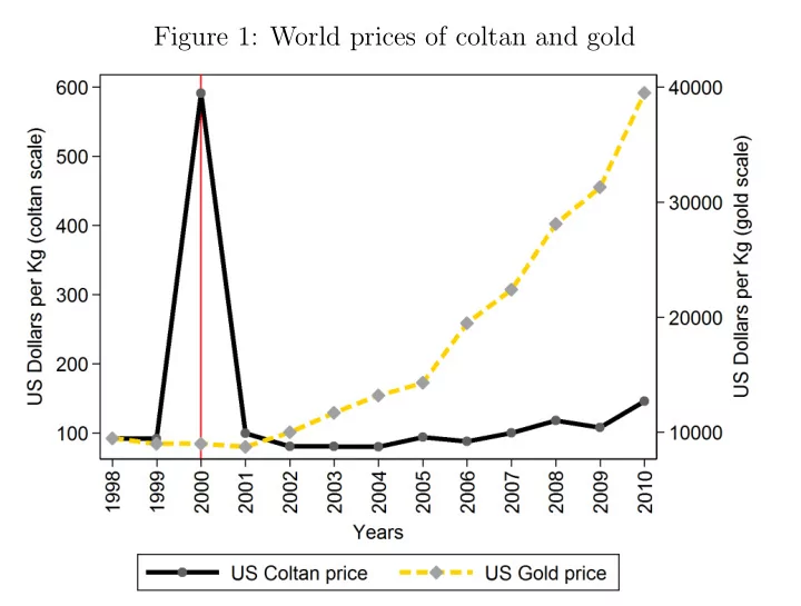
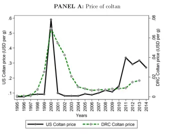
Figure 1: World prices of coltan and gold Figure 2: Local prices of - PowerPoint PPT Presentation
Figure 1: World prices of coltan and gold Figure 2: Local prices of coltan and gold Figure 6: Demand shock for coltan and presence of stationary bandits Notes : This figure plots the average number of stationary bandits on year. I take the
Figure 1: World prices of coltan and gold
Figure 2: Local prices of coltan and gold
Figure 6: Demand shock for coltan and presence of stationary bandits Notes : This figure plots the average number of stationary bandits on year. I take the variable stationary bandit from the site survey, in which the specialists are asked to list past “organizations of security” in the site. A stationary bandit (“organization of security” in the survey) is defined as an armed actor who holds the monopoly of violence in a given site for at least 6 months (approximately). Stationary bandits most frequently are alone when they occupy a site. In some cases, multiple stationary bandits collude (this is mostly the case for the Mayi-Mayis and the FDLR in some cases), and in some, fewer cases, more than one stationary bandit may alternate in one location in a given year. The solid line graphs the average number of stationary bandits per year for mining sites that are endowed with coltan deposits, and the dashed line reports the same quantity for mining sites not endowed with coltan deposits.
Table 2: Effects of price shocks, presence of stationary bandit (1) (2) (3) (4) (5) (6) (7) (8) (9) VARIABLES Coltan(i) X pc(t) 0.07** 0.10*** 0.17*** 0.21*** 0.11*** 0.20*** 0.12*** 0.13** 0.28*** (0.03) (0.03) (0.04) (0.05) (0.03) (0.03) (0.02) (0.05) (0.08) Coltan(i) X pc(t) X D road(i) -0.08 -0.07 (0.07) (0.07) pc(t) X D road(i) 0.03 0.03 (0.03) (0.04) Gold(i) X pg(t) -0.03 (0.03) Coltan(i) X pc(t) X D airport(i) -0.13** -0.10 (0.06) (0.06) pc(t) X D airport(i) 0.01 0.00 (0.02) (0.04) Coltan(i) X pc(t+1) 0.06** (0.03) Constant 0.27** 0.29*** 0.17* 0.20*** 0.27*** -0.03 0.00 41.97 91.16* (0.11) (0.06) (0.09) (0.07) (0.06) (0.10) (0.00) (46.28) (49.25) Observations 2,134 388 360 360 388 582 388 582 540 R-squared 0.68 0.87 0.87 0.88 0.88 0.76 0.79 0.82 Year FE YES YES YES YES YES YES YES YES YES Village FE YES YES YES YES YES YES YES YES YES Region*Year FE NO NO NO NO YES YES NO NO YES Arellano-Bond NO NO NO NO NO NO YES NO NO Coltan time trends NO NO NO NO NO NO NO YES YES Sample 98-08 99-00 99-00 99-00 99-00 98-00 98-00 98-00 98-00
Figure 7: Effect of the price of gold on stationary bandits at gold sites, all time intervals Notes : This figure plots the estimated coefficients on gold endowment, interacted with the world price of gold, from the baseline specification using all possible time intervals. Intervals indicate 95% confidence intevals.
Figure 8: Effect of the price of coltan on stationary bandits at coltan sites, all time intervals Notes : This figure plots the estimated coefficients on coltan endowment, interacted with the world price of coltan, from the baseline specification using all possible time intervals. Intervals indicate 95% confidence intevals.
Figure 9: Demand shock for coltan and presence of taxation Notes : This figure plots the average number of sites where an armed actor collects taxes regularly on years. I take this variable from the site survey, in which the specialists are asked to list past taxes in the site. Taxes by an armed actor are defined in the survey as a mandatory payment on mining activity which is regular (sporadic expropriation is excluded), stable (rates of expropriation are stable) and anticipated (villagers make investment decisions with knowledge of these expropriation rates and that these will be respected). The solid line graphs the average number of mining sites where an armed actor collects regular taxes for mining sites that are endowed with available coltan deposits, and the dashed line reports the same quantity for mining sites that are not endowed with coltan deposits.
Table 3: Effects of price shocks, presence of taxation (1) (2) (3) (4) (5) (6) (7) (8) (9) VARIABLES Coltan(i) X pc(t) 0.15*** 0.17*** 0.19*** 0.29*** 0.18*** 0.23*** 0.07*** 0.16*** 0.29*** (0.03) (0.04) (0.05) (0.06) (0.04) (0.03) (0.01) (0.06) (0.08) Coltan(i) X pc(t) X D road(i) -0.01 0.01 (0.08) (0.07) pc(t) X D road(i) 0.01 -0.02 (0.02) (0.03) Gold(i) X pg(t) 0.01 (0.03) Coltan(i) X pc(t) X D airport(i) -0.17** -0.22*** (0.08) (0.06) pc(t) X D airport(i) -0.00 0.07 (0.03) (0.05) Coltan(i) X pc(t+1) 0.05 (0.03) Constant -0.16 -0.11 -0.17 -0.14 -0.13 -0.36*** 0.00 -28.71 -11.57 (0.11) (0.09) (0.10) (0.09) (0.08) (0.12) (0.00) (54.65) (57.61) Observations 1,417 258 240 240 258 385 256 385 358 R-squared 0.71 0.84 0.85 0.86 0.86 0.77 0.77 0.82 Year FE YES YES YES YES YES YES YES YES YES Village FE YES YES YES YES YES YES YES YES YES Region*Year FE NO NO NO NO YES YES NO NO YES Arellano-Bond NO NO NO NO NO NO YES NO NO Coltan time trends NO NO NO NO NO NO NO YES YES Sample 98-08 99-00 99-00 99-00 99-00 98-00 98-00 98-00 98-00
Table 4: Effects of price shocks by type of tax (1) (2) (3) (4) (5) (6) (7) Output Labor Poll Food Transit Mill Pillage VARIABLES Tax Tax Tax Tax Tax Tax Coltan(i) X pc(t) 0.12*** 0.07*** 0.10*** -0.01 0.01 0.02 -0.04 (0.03) (0.02) (0.03) (0.02) (0.03) (0.02) (0.04) Constant -0.20*** -0.06 0.28*** 0.11** 0.13** 0.01 0.24*** (0.06) (0.06) (0.07) (0.05) (0.06) (0.03) (0.09) Observations 1,521 1,599 1,690 1,463 1,729 1,729 1,729 R-squared 0.60 0.72 0.56 0.61 0.59 0.72 0.12 Year FE YES YES YES YES YES YES YES Village FE YES YES YES YES YES YES YES Location MINE MINE VILLAGE MARKET VILLAGE VILLAGE VILLAGE Sample 99-00 99-00 99-00 99-00 99-00 99-00 99-00
Recommend
More recommend
Explore More Topics
Stay informed with curated content and fresh updates.




![Figure 1: Team Logo 2 Figure 2: AISC SSBC Event Logo [1] Figure 3: Vertical Load locations [1]](https://c.sambuz.com/492196/figure-1-team-logo-s.webp)
