Log-Linear Models Noah A. Smith Department of Computer Science / - PDF document
Log-Linear Models Noah A. Smith Department of Computer Science / Center for Language and Speech Processing Johns Hopkins University nasmith@cs.jhu.edu December 2004 Abstract This is yet another introduction to log-linear (maximum
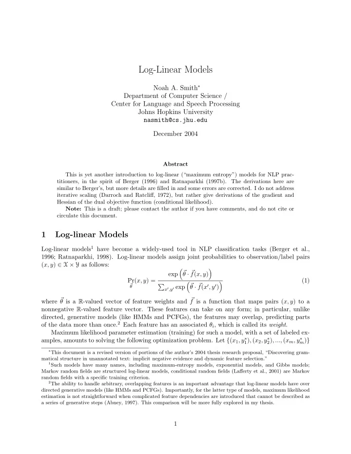
Log-Linear Models Noah A. Smith ∗ Department of Computer Science / Center for Language and Speech Processing Johns Hopkins University nasmith@cs.jhu.edu December 2004 Abstract This is yet another introduction to log-linear (“maximum entropy”) models for NLP prac- titioners, in the spirit of Berger (1996) and Ratnaparkhi (1997b). The derivations here are similar to Berger’s, but more details are filled in and some errors are corrected. I do not address iterative scaling (Darroch and Ratcliff, 1972), but rather give derivations of the gradient and Hessian of the dual objective function (conditional likelihood). Note: This is a draft; please contact the author if you have comments, and do not cite or circulate this document. 1 Log-linear Models Log-linear models 1 have become a widely-used tool in NLP classification tasks (Berger et al., 1996; Ratnaparkhi, 1998). Log-linear models assign joint probabilities to observation/label pairs ( x, y ) ∈ X × Y as follows: � � � θ · � exp f ( x, y ) Pr ( x, y ) = (1) � � � � θ · � � f ( x ′ , y ′ ) x ′ ,y ′ exp θ where � θ is a R -valued vector of feature weights and � f is a function that maps pairs ( x, y ) to a nonnegative R -valued feature vector. These features can take on any form; in particular, unlike directed, generative models (like HMMs and PCFGs), the features may overlap, predicting parts of the data more than once. 2 Each feature has an associated θ i , which is called its weight . Maximum likelihood parameter estimation (training) for such a model, with a set of labeled ex- amples, amounts to solving the following optimization problem. Let { ( x 1 , y ∗ 1 ) , ( x 2 , y ∗ 2 ) , ..., ( x m , y ∗ m ) } ∗ This document is a revised version of portions of the author’s 2004 thesis research proposal, “Discovering gram- matical structure in unannotated text: implicit negative evidence and dynamic feature selection.” 1 Such models have many names, including maximum-entropy models, exponential models, and Gibbs models; Markov random fields are structured log-linear models, conditional random fields (Lafferty et al., 2001) are Markov random fields with a specific training criterion. 2 The ability to handle arbitrary, overlapping features is an important advantage that log-linear models have over directed generative models (like HMMs and PCFGs). Importantly, for the latter type of models, maximum likelihood estimation is not straightforward when complicated feature dependencies are introduced that cannot be described as a series of generative steps (Abney, 1997). This comparison will be more fully explored in my thesis. 1
be the labeled training set. m � � θ ∗ ( x j , y ∗ = max Pr j ) (2) � � θ θ j =1 m � log Pr � θ ( x j , y ∗ = max j ) (3) � θ j =1 � � θ · � � f ( x j , y ∗ m exp j ) (Eq. 1) � = max log (4) � �� � � θ · � � f ( x ′ , y ′ ) x ′ ,y ′ exp θ � � � j =1 Z θ m � � θ · � f ( x j , y ∗ − m log Z ( � = j ) θ ) (5) j =1 This function can be shown to be concave, with a single global maximum. 3 Commonly the conditional probability of the label given the observation is computed; for one example ( x, y ) it is given by: � � � θ · � exp f ( x, y ) Pr ( y | x ) = (6) � � � � θ · � � f ( x, y ′ ) y ′ exp θ Why is this quantity important? A second feature of log-linear models is that they admit relatively efficient conditional parameter estimation. Conditional training is a technique that seeks to give maximum probability (or weight, or score) to the correct label y ∗ for a given observation x (known from an annotated corpus), at the expense of competing possible labels. This kind of training can be contrasted with joint maximum likelihood training (Equation 4), which seeks to maximize the total probability of training pairs ( x j , y ∗ j ). Conditional training for log-linear models amounts to maximizing the product of conditional probabilities (as in Equation 6): 4 m � � θ ∗ ( y ∗ = max Pr j | x j ) (7) � � θ θ j =1 m � ( y ∗ = max log Pr j | x j ) (8) � � θ θ j =1 m m � � � � � � θ · � θ · � � f ( x j , y ∗ − f ( x j , y ′ ) = j ) log exp (9) j =1 j =1 y ′ � �� � Z ( � θ,x j ) The argument for conditional training is that it is unnecessary to model x , the observed part of the data, since (even at test time) it is given; we need only be able to determine which y fits x 3 In Section 3 I derive the Hessian and demonstrate that the function is everywhere concave. 4 A discussion of conditional likelihood as a statistical estimator is given by Johnson et al. (1999). An earlier discussion is Nadas (1983). 2
best, and predicting x is extraneous effort imposed on the model. 5 θ ( y ∗ | x ) rather than Pr � θ ( x, y ∗ ). There is also a practical reason for using conditional likelihood Pr � Consider the terms marked in Equations 4 and 9 as Z ( � θ ) and Z ( � θ, x j ), respectively. This term is known as the partition function . In ML training (Equation 4), computing it involves summing over the entire space of observation/label pairs predicted by the model, while in conditional training (Equation 9) one must sum only over the labels for each example x . The former is in practice much more computationally expensive, even with approximations. Both optimization problems are unconstrained and convex, making them relatively straightfor- ward to solve (modulo the partition function) using iterative hill-climbing methods. Iterative scaling (Darroch and Ratcliff, 1972) is one approach; Malouf (2002) describes how Newtonian numerical optimization algorithms using the gradient of the function can be used (see Section 3). 6 With log-linear models of labeled data, the numerical part of learning is straightforward; the difficult part is feature selection. Using too many features is likely to result in over-fitting of the training data. One approach is to use features that have frequency in training data above some threshold; Della Pietra et al. (1997) use a more sophisticated feature selection algorithm. Another way of avoiding over-fitting is to smooth the model. This is often done using a prior (Khudanpur, 1995; Chen and Rosenfeld, 2000). One recent approach to smoothing by Kazama and Tsujii (2003) (this work extends that of Khudanpur (1995)) uses soft constraints and a penalty function (which can be interpreted as a prior on parameter values); this has the side-effect of many parameters going to zero, 7 resulting in automatic feature selection. 8 Of course, introducing priors requires introducing more parameters (and perhaps auxiliary learning algorithms to estimate them). This is an active area of research. Log-linear models have been applied to many supervised problems in NLP: • Sentence boundary detection (Reynar and Ratnaparkhi, 1997) • Parsing (Ratnaparkhi et al., 1994b; Ratnaparkhi, 1997a; Abney, 1997; Riezler et al., 2000; Johnson and Riezler, 2000; Johnson, 2001) 9 5 Conditional training encompasses a number of approaches to parameter estimation and originated in the auto- matic speech recognition community. In particular, maximum mutual information (MMI) estimation (Bahl et al., 1986) can be shown to be equivalent to conditional maximum likelihood estimation. The other approach is to directly minimize classification error (Juang and Katagiri, 1992). 6 The learning task for log-linear models is usually described as follows. Given a vector of observed feature values ˜ f , we seek model parameters � � θ that yield these expectations. That is, we wish the following constraint to be met for all feature indices i : ( y | x ) f i ( x, y ) = ˜ � Pr (10) f i . � θ x,y Now, there may be many solutions to this system of equations. The criterion used to decide among them is maximum entropy — we seek the parameters that are closest to uninformative (uniform), subject to the expectation constraints. This is motivated by an Occam’s razor argument that advocates choosing the simplest possible model that explains the data; entropy can be roughly regarded as a measure of simplicity of the model. It turns out that the dual of this constrained optimization problem has the form of the maximum likelihood problems given in Equations 4 and 9, depending on whether the entropy to be maximized is joint entropy H (Pr � θ ( X, Y )) or the total entropy of the conditional distributions for each x j , � m j =1 H (Pr � θ ( Y | x j )) (Berger et al., 1996). See Section 2 for a derivation of the dual in the latter case. 7 A zero-weighted feature will have no effect on the probability of examples where the feature is present; see Equation 1. 8 To my knowledge, this technique has not been carefully tested as a feature selection technique per se , though M. Osborne (personal communication) reports that its performance as such is reasonable in comparison with other feature selection algorithms. 9 Charniak (2000) used log-linear-like features to build a state-of-the-art parser, but without training via the 3
Recommend
More recommend
Explore More Topics
Stay informed with curated content and fresh updates.
![(142733/102960-Log[4])+(614851/73920-2 Log[64]) h 2 +(2329/1680-Log[4]) h 4 -h 10 /20160](https://c.sambuz.com/761724/142733-102960-log-4-614851-73920-2-log-64-h-2-2329-1680-s.webp)
