Functional Linear Models 1 66 / 181 Functional Linear Models - PowerPoint PPT Presentation

Functional Linear Models Functional Linear Models 1 66 / 181

Functional Linear Models Statistical Models So far we have focussed on exploratory data analysis Smoothing Functional covariance Functional PCA Now we wish to examine predictive relationships → generalization of linear models. � y i = α + β j x ij + ǫ i 67 / 181 2

Functional Linear Models Functional Linear Regression y i = α + x i β + ǫ i Three different scenarios for y i x i Functional covariate, scalar response Scalar covariate, functional response Functional covariate, functional response We will deal with each in turn. 68 / 181 3

Functional Linear Models: Scalar Response Models Scalar Response Models 4 69 / 181

Functional Linear Models: Scalar Response Models In the Limit If we let t 1 , . . . get increasingly dense � y i = α + β j x i ( t j ) + ǫ i = α + x i β + ǫ i becomes � y i = α + β ( t ) x i ( t ) dt + ǫ i General trick: functional data model = multivariate model with sums replaced by integrals. Already seen in fPCA scores x T u i → � x ( t ) ξ i ( t ) dt . 71 / 181 5 Generalization of multiple linear regression

Functional Linear Models: Scalar Response Models Identification Problem: In linear regression, we must have fewer covariates than observations. If I have y i , x i ( t ) , there are infinitely many covariates. � y i = α + β ( t ) x i ( t ) dt + ǫ i Estimate β by minimizing squared error: � 2 � � � β ( t ) = argmin y i − α − β ( t ) x i ( t ) dt But I can always make the ǫ i = 0. 72 / 181 6

Functional Linear Models: Scalar Response Models Smoothing Additional constraints: we want to insist that β ( t ) is smooth. Add a smoothing penalty: n � 2 � � � [ L β ( t )] 2 dt � PENSSE λ ( β ) = y i − α − β ( t ) x i ( t ) dt + λ i = 1 Very much like smoothing (can be made mathematically precise). Still need to represent β ( t ) – use a basis expansion: � β ( t ) = c i φ i ( t ) . 7 73 / 181

Functional Linear Models: Scalar Response Models Calculation �� � � y i = α + β ( t ) x i ( t ) dt + ǫ i = α + Φ( t ) x i ( t ) dt c + ǫ i = α + x i c + ǫ i � for x i = Φ( t ) x i ( t ) dt . With Z i = [ 1 x i ] , � α � y = Z + ǫ c and with smoothing penalty matrix R L : � − 1 c T ] T = � Z T Z + λ R L Z T y [ˆ α ˆ Then � ˆ � � α ˆ ˆ y = β ( t ) x i ( t ) dt = Z = S λ y ˆ c 8 74 / 181

Functional Linear Models: Scalar Response Models Choosing Smoothing Parameters Cross-Validation: � 2 � � y i − ˆ y i OCV ( λ ) = 1 − S ii λ = e − 1 λ = e 20 λ = e 12 CV Error 75 / 181 9

Functional Linear Models: Scalar Response Models Confidence Intervals Assuming independent ǫ i ∼ N ( 0 , σ 2 e ) We have that � ˆ � �� � � � � � − 1 � α � − 1 � Z T Z + λ R Z T σ 2 Z T Z + λ R Var = Z e I ˆ c Estimate σ 2 ˆ e = SSE / ( n − df ) , df = trace ( S λ ) And (pointwise) confidence intervals for β ( t ) are � Φ( t )ˆ c ± 2 Φ( t ) T Var [ˆ c ]Φ( t ) 76 / 181 10

Functional Linear Models: Scalar Response Models Confidence Intervals R 2 = 0 . 987 σ 2 = 349, df = 5.04 Extension to multiple functional covariates follows same lines: p � � y i = β 0 + β j ( t ) x ij ( t ) dt + ǫ i j = 1 11 77 / 181

Functional Linear Models: functional Principal Components Regression functional Principal Components Regression Alternative: principal components regression. � � x i ( t ) = d ij ξ j ( t ) d ij = x i ( t ) ξ j ( t ) dt Consider the model: � y i = β 0 + β j d ij + ǫ i Reduces to a standard linear regression problem. Avoids the need for cross-validation (assuming number of PCs is fixed). By far the most theoretically studied method. 79 / 181 12

Functional Linear Models: functional Principal Components Regression fPCA and Functional Regression Interpretation � y i = β 0 + β j d ij + ǫ i � Recall that d ij = x i ( t ) ξ j ( t ) dt so � � y i = β 0 + β j ξ j ( t ) x i ( t ) dt + ǫ i and we can interpret � β ( t ) = β j ξ j ( t ) and write � y i = β 0 + β ( t ) x i ( t ) dt + ǫ i Confidence intervals derive from variance of the d ij . 80 / 181 13

Functional Linear Models: functional Principal Components Regression A Comparison Medfly Data: fPCA on 4 components ( R 2 = 0 . 988) vs Penalized Smooth ( R 2 = 0 . 987) 14 81 / 181

Advantages of FPCA-based approach Parsimonious description of functional data as it is the unique linear representation which explains the highest fraction of variance in the data with a given number of components. Main attraction is equivalence X ( · ) ∼ ( ξ 1 , ξ 2 , · · · ), so that X ( · ) can be expressed in terms of mean function and the sequence of eigenfunctions and uncorrelated FPC scores ξ k ’s. For modeling functional regression: Functions f { X ( · ) } have an equivalent function g ( ξ 1 , ξ 2 , · · · ) But need to pay prices FPCs need to be estimated from data (finite sample) Need to choose the number of FPCs 15

Functional Linear Models: functional Principal Components Regression Two Fundamental Approaches (Almost) all methods reduce to one of 1 Perform fPCA and use PC scores in a multivariate method. 2 Turn sums into integrals and add a smoothing penalty. Applied in functional versions of generalized linear models generalized additive models survival analysis mixture regression ... Both methods also apply to functional response models. 16 82 / 181

Functional Linear Models: Functional Response Models Functional Response Models 83 / 181 17

Functional Linear Models: Functional Response Models Functional Response Models Case 1: Scalar Covariates: ( y i ( t ) , x i ) , most general linear model is p � y i ( t ) = β 0 ( t ) + β i ( t ) x ij . j = 1 Conduct a linear regression at each time t (also works for ANOVA effects). But we might like to smooth; penalize integrated squared error n p � � y i ( t )) 2 dt + [ L j β j ( t )] 2 dt � � PENSISE = ( y i ( t ) − ˆ λ j i = 1 j = 0 Usually keep λ j , L j all the same. 84 / 181 18

Functional Linear Models: Functional Response Models Concurrent Linear Model Extension of scalar covariate model: response only depends on x ( t ) at the current time y i ( t ) = β 0 ( t ) + β 1 ( t ) x i ( t ) + ǫ i ( t ) y i ( t ) , x i ( t ) must be measured on same time domain. Must be appropriate to compare observations time-point by time-point (see registration section). Especially useful if y i ( t ) is a derivative of x i ( t ) (see dynamics section). 19 85 / 181

Functional Linear Models: Functional Response Models Functional Response, Functional Covariate General case: y i ( t ) , x i ( s ) - a functional linear regression at each time t : � y i ( t ) = β 0 ( t ) + β 1 ( s , t ) x i ( s ) ds + ǫ i ( t ) Same identification issues as scalar response models. Usually penalize β 1 in each direction separately � � [ L s β 1 ( s , t )] 2 dsdt + λ t [ L t β 1 ( s , t )] 2 dsdt λ s Confidence Intervals etc. follow from same principles. 20 90 / 181

Functional Linear Models: Functional Response Models Summary Three models Scalar Response Models Functional covariate implies a functional parameter. Use smoothness of β 1 ( t ) to obtain identifiability. Variance estimates come from sandwich estimators. Concurrent Linear Model y i ( t ) only depends on x i ( t ) at the current time. Scalar covariates = constant functions. Will be used in dynamics. Functional Covariate/Functional Response Most general functional linear model. See special topics for more + examples. 91 / 181 21

Other Topics and Recent Developments Inference for functional regression models Dependent functional data – Multilevel/longitudinal/multivariate designs Registratoin Dynamics FDA for sparse longitudinal data More general/flexible regression models 22

Inference for functional regression models Testing H 0 : β ( t ) = 0 under model � Y i = β 0 + β ( t ) X i ( t ) dt + ǫ i Penalized spline approach β ( t ) = � M m =1 η k B k ( t ) FPCA-based approach data reduction: ( ξ i 1 , · · · , ξ iK ) multivariate regression: Y i ∼ β 1 ξ i 1 + · · · + β K ξ iK Difficulty in inference arising from regularization (smoothing) choices of tuning parameters accounting for uncertainly in two-step procedures 23

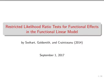
Penalized spline approach H 0 : η 0 = η 1 = · · · = η M β ( t ) 2 dt to avoid overfitting � Use roughness penalty λ Mixed model equivalence representation M � Y i = β 0 + η m V im + ǫ i m =1 ( η 1 , · · · , η M ) ∼ N (0 , σ 2 Σ) Testing H 0 : σ 2 = 0 Restricted LRT proposed in the literature. Swihart, Goldsmith and Crainiceanu (2014). Restricted likelihood ratio tests for functional effects in the functional linear model. Technometrics, 56:483–493. 24

FPCA-based approach Y i ∼ β 1 ξ i 1 + · · · + β K ξ iK Testing H 0 : β 1 = · · · = β K = 0 The number of PCs are chosen by Percent of variance explained (PVE): e.g., 95% or 99% Cross Validation AIC, BIC Wald test K K Y T ˆ ˆ ξ k ˆ β 2 ξ T 1 k Y � � ∼ χ 2 k T = = K var(ˆ σ 2 ˆ n ˆ ˆ β k ) λ k ǫ k =1 k =1 But is it a good idea to rank based on X ( t ) only? And how sensitive is the power to the choice of K? 25