A new method for the detemination of the charge of the Top: - PDF document

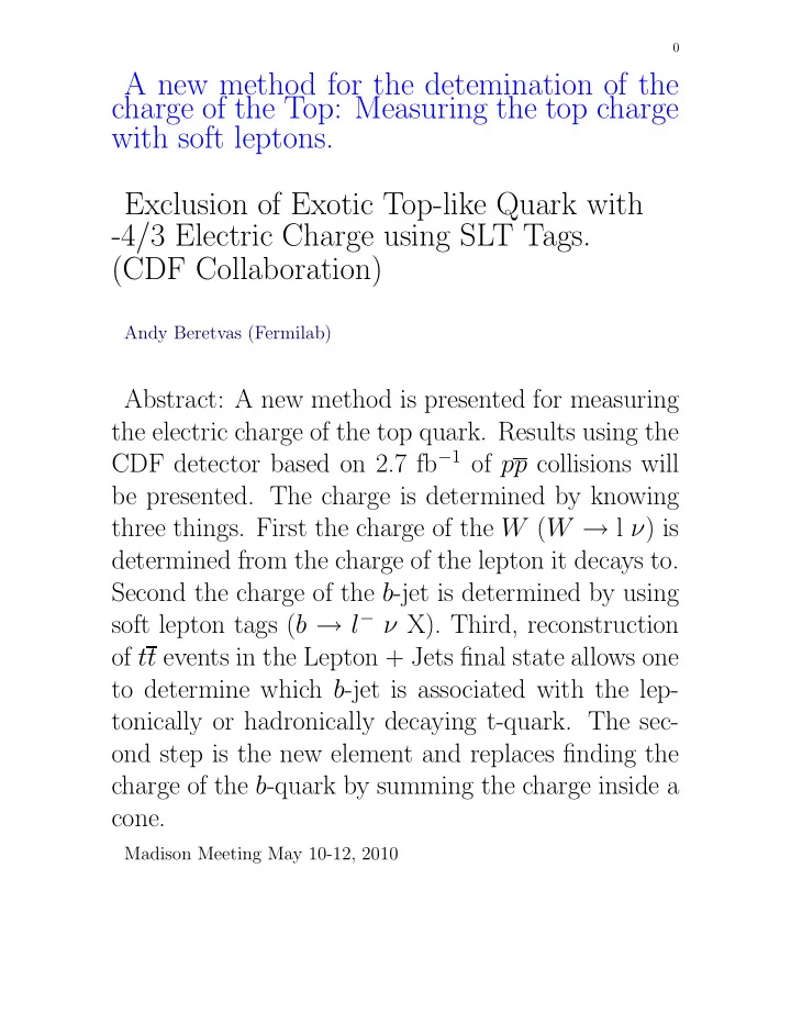
0 A new method for the detemination of the charge of the Top: Measuring the top charge with soft leptons. Exclusion of Exotic Top-like Quark with -4/3 Electric Charge using SLT Tags. (CDF Collaboration) Andy Beretvas (Fermilab) Abstract: A new method is presented for measuring the electric charge of the top quark. Results using the CDF detector based on 2.7 fb − 1 of pp collisions will be presented. The charge is determined by knowing three things. First the charge of the W ( W → l ν ) is determined from the charge of the lepton it decays to. Second the charge of the b -jet is determined by using soft lepton tags ( b → l − ν X). Third, reconstruction of tt events in the Lepton + Jets final state allows one to determine which b -jet is associated with the lep- tonically or hadronically decaying t-quark. The sec- ond step is the new element and replaces finding the charge of the b -quark by summing the charge inside a cone. Madison Meeting May 10-12, 2010

1 Exclusion of Exotic Top-like Quark with -4/3 Electric Charge using SLT Tags. (CDF Collaboration) Outline of Talk 1. Standard Model versus Exotic Model 2. Determining the Charge of the Top Quark 3. Obtaining a clean sample 4. Basic Statistical Elements N pairs Purity pair Binominal Distribution 5. How many pairs? 6. Statistical errors α and β 7. Need a Hypothesis to Test 8. Results 9. Conclusions Outline Madison Meeting May 10-12, 2010

2 1. Standard Model versus Exotic Model Basic Question for this Analysis tt → W + b W − b (SM) standard model tt → W − b W + b (XM) exotic model We use the lepton plus jet decay mode (L+J) tt → ( l + ν b ) ( qq b ) (SM) standard model tt → ( l − ν b ) ( qq b ) (XM) exotic model The leptons used are e and µ We use a kinematic fitter to tell which b is associated (paired) with the lepton • SM Charge of lepton is opposite to the charge of the paired b • XM Charge of lepton is the same as the charge of the paired b Slide 2 Madison Meeting May 10-12, 2010

3 2. Determining the Charge of the Top Quark • Correct pairing of lepton and b Kinematic Fitter (Purity = P k = 76%) Kinematic Fitter = Reconstruction technique that assigns jets to their partons • Charge of the lepton • Charge of the b Standard Method of Determining the Charge of the b The determination of the flavor of a b jet is based on jet charge calculation. The charges of tracks inside a jet (cone of radius = 0.4 in η - φ space) are summed up with weights defined by momentum amplitude of the track and the closeness of the track to the jet axis. � | � p i . � P jet | 0 . 5 Q i Q jet = (1) � | � p i . � P jet | 0 . 5 Where � p i , Q i is momentum and charge of a track � associated with a jet and P jet , Q jet momentum and charge of the jet. Slide 3 Madison Meeting May 10-12, 2010

4 • Charge of the b Purity tagger = P t = 71% New Method of Determining the Charge of the b Semileptonic Decay Mode • b → l − νX • b → l + νX Not easy, one needs to identify electrons embeded in jets. FIG. 1: Predicted efficiency to tag an electron from semileptonic decay of HF and a hadron candidate SLT e track in t ¯ t events as a function of the track p T (a) and corrected jet E T (b). The left axis indicates the tagging efficiency for the electrons and the right axis indicates the tagging efficiency for the hadrons. Slide 4 Madison Meeting May 10-12, 2010

5 3. Obtaining a clean Sample • We would like no Background • We get a Signal/Background = 12.5/1 • soft lepton tag (SLT) • standard secondary vertex tag (SECVTX) • high p T leptons ( p T > 20 GeV) • lepton must be central ( | η | ) < 1. • lepton must be isolated ( > 90% of Energy in cone of R = 0.4) • E T / > 30 GeV • Three or more high E T jets • The fourth jet can be lower ( E T > 12 GeV) • H T > 200 GeV (Scaler sum of transverse energy of leptons, jets and neutrinos) • χ 2 constraint on kinematic fitter • Reject events containing cosmic muons • Reject conversion electrons • Reject events containing a Z • Reject events with more than one high p T lepton Slide 5 Madison Meeting May 10-12, 2010

6 4. Basic Statistical Elements • Two Important Quantaties (Number of Events, Purity) • Number of Signal Events (I assume only one SLT in an event) N SM • Purity = P = N SM +N XM • Purity SLT Tagger = P t = 71% • Purity Kinematic Fitter = P k = 76% • P = P k P t + (1. - P k )(1. - P t ) = 61% • The figure of Merit for the experiment = ǫ D 2 N SM • For the SM, ǫ = N pre − tag • Dilution = D = 2P - 1 If you are interested in the XM model replace N SM with N XM and N XM with N SM Slide 6 Madison Meeting May 10-12, 2010

7 5. How many pairs? • Branching Fraction for: tt → Lepton + Jets( e + µ ) = 29.6% • Pretag Acceptance = ǫ pretag = 29.6%*0.21 = 6.2% • ǫ trigger = 0.96, We collect events that fire an inclusive 8 GeV trigger • (SF = 0.92) to correct between MC and Data, ǫ Dilution(Data) = SF 2 ǫ Dilution(MC) = 0.85 • The square is because we need to correct both the lepton-jet and the away-jet • Pretag Acceptance(corrected) ǫ pretag − c = 6.2% × ǫ trigger × ǫ Dilution = 5.1% • N pretag = ǫ pretag − c × σ ( tt ) × L • N pretag = 5.1% × 6.7pb × 2700/pb = 922 • ǫ tag ( SLT and SECVTX ) = 3.2% • N SLT+SECVTX = N pretag ǫ tag = 922 × 0.032 = 30. • Why is ǫ ( tag SLT and SECVTX) so small ? • Branching Fraction( b → lνX ) ≈ = 10% • Kinematic Fitter both b ’s are tagged ( χ 2 < 27) or both tags on the same b ( χ 2 < 9) • p T ( Soft Lepton ) > 6 GeV • p T ( Soft Muons(relative to the jet axis)) > 1.5 GeV Slide 7 Madison Meeting May 10-12, 2010

8 • How many background pairs? TABLE I: Process pretag SM + XM Tags Diboson 73.23 ± 4.04 0.13 ± 0.01 Single Top 14.25 ± 0.83 0.24 ± 0.01 Z + Jets 63.85 ± 10.35 0.31 ± 0.06 Drell-Yan 14.08 ± 2.95 0.06 ± 0.01 QCD 198.91 ± 31.96 0.00 ± 0.43 W + LF 0.25 ± 0.04 W + bb 1.07 ± 0.29 W + cc / W + c 0.31 ± 0.07 W + Jets 1067.08 ± 149.46 (1.64 ± 0.30) Total Background 1431.41 ± 133.13 2.36 ± 0.52 • Total sample size 30. (Signal) + 2.36 (Background) ≈ 32. • Total Purity 0.608 (Signal) + 0.5 (Background) ≈ 0.60 Slide 8 Madison Meeting May 10-12, 2010

9 6. Statistical Errors α and β • Type I Errors called alpha • Type II Errors called beta • In a legal proceeding: • One would say the probability of an innocent person going to jail is alpha. • The probability of a guilty person going free is beta • Clearly one wants both alpha and beta to be as small as possible • http://www.intuitor.com/statistics/T1T2Errors.html • A pregency test: • If the test says a women is pregnant when she is not, this is a type I error (alpha). • Type II error (beta) is when a test shows a women is not pregnant when she is. • Clearly one wants both alpha and beta to be as small as possible These questions about statistics have been around for a long time. J. Neyman and E. Pearson Phil. Trans. of the Royal Soc. of London A31 289 (1933). Slide 9 Madison Meeting May 10-12, 2010

10 7. Need a Hypothesis to Test • What do we need to know in order to proceed. • We must have a hypothesis (H 0 ) The person is innocent. The women is pregnant The exotic model is true. • We must know the probability distributions for both alter- nativces. Probability distributions for the legal case ? Probability distributions for the medical case ? For our case it’s just the Binominal distribution (p + q) n For SM we have p = 0.6 and q = 0.4, n = 30 • We need to set alpha before we do the experiment • There are four standard choices 95%, 99%, 3 σ and 5 σ • For Top charge analysis we will choose 95% (alpha =5%) Are we proceeding correctly? Yes but, physics could be strange 50% charge 2/3 and 50% charge -4/3 Slide 10 Madison Meeting May 10-12, 2010

11 • H 0 = The exotic Model is true TABLE II: This table represents our understanding before doing the experiment. Result of Test H 0 true H 0 false Do not reject H 0 OK-1 Type I error Reject H 0 Type II error OK-2 • We plot both distributions (SM and XM), and draw a line so that (XM) exotic distribution has 95% of its area to the left of the line. The 5% to the right corresponds to alpha. • To determine beta we use the same line, but look at the SM distribution. The area to the left of the line corresponds to beta, the area to the right is 1 - β ( Sometimes called the power of the method.) TABLE III: This table represents our understanding before doing the experiment. Result of Test XM true XM false Do not reject XM 95% 5% Reject XM 28.6% 71.4% • If we reject the Hypothesis we will publish a 95% CL of excluding the XM model. • If we do not reject the Hypothesis we will look at the alter- native hypothesis. Slide 11 Madison Meeting May 10-12, 2010

12 8. Results h1 h1 Distribution for SLT (SM black) for N = 30 and p = 0.6 Entries Entries 31 31 1 Mean Mean 0.4032 0.4032 CDF Preliminary RMS 0.08656 RMS 0.08656 Measurement 11 13 -1 10 9 15 7 17 -2 10 19 5 10 -3 21 3 -4 10 0 0.1 0.2 0.3 0.4 0.5 0.6 0.7 0.8 0.9 1 Purity FIG. 2: The blue line has approximately 5% of the XM curve to it’s right. • If we observe 17 or more SM pairs out of 30 we will have excluded the XM model at a 95% CL. • We observe 19.3 • The reason for the strange number is that we re- constructed 45 events (SM = 29, XM = 16) Slide 12 Madison Meeting May 10-12, 2010