Hypothesis Testing in Regression Models Recall the regression model: - - PowerPoint PPT Presentation

▶

Sep 14, 2023 301 likes •493 views

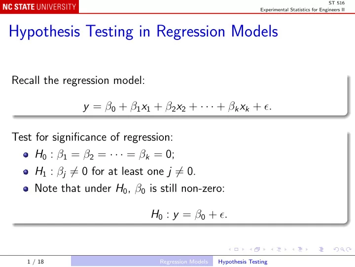
ST 516 Experimental Statistics for Engineers II Hypothesis Testing in Regression Models Recall the regression model: y = 0 + 1 x 1 + 2 x 2 + + k x k + . Test for significance of regression: H 0 : 1 = 2 = =

SLIDE 1

ST 516 Experimental Statistics for Engineers II

Hypothesis Testing in Regression Models

Recall the regression model: y = β0 + β1x1 + β2x2 + · · · + βkxk + ǫ. Test for significance of regression: H0 : β1 = β2 = · · · = βk = 0; H1 : βj = 0 for at least one j = 0. Note that under H0, β0 is still non-zero: H0 : y = β0 + ǫ.

1 / 18 Regression Models Hypothesis Testing

SLIDE 2

ST 516 Experimental Statistics for Engineers II

The ANOVA table: Source SS df MS F0 Regression SSR k MSR MSR/MSE Error SSE n − k − 1 MSE Total SST n − 1 Here, as before, SSE is the residual sum of squares, SSE =

(yi − ˆ yi)2 =

e2

i = e′e = y′y − ˆ

β

′X′y.

2 / 18 Regression Models Hypothesis Testing

SLIDE 3

ST 516 Experimental Statistics for Engineers II

Also SST is the total sum of squares, SST =

(yi − ¯ y)2 , and the regression sum of squares is SSR =

(ˆ yi − ¯ y)2 = SST − SSE. Test statistic: F0 = SSR/k SSE/(n − k − 1) = SSR/k SSE/(n − p) = MSR MSE . Assuming ǫs are NID(0, σ2), reject H0 if F0 > Fα,k,n−p.

3 / 18 Regression Models Hypothesis Testing

SLIDE 4

ST 516 Experimental Statistics for Engineers II

Note: under H0, y = β0 + ǫ, so y has a non-zero mean, but no dependence on any of the regressors. F0 is calculated and reported by all packages.

4 / 18 Regression Models Hypothesis Testing

SLIDE 5

ST 516 Experimental Statistics for Engineers II

Also calculated: the coefficient of multiple determination R2 = SSR SST = 1 − SSE SST . Note: R2 always increases if you add a new regressor to a model, so high R2 may result from including too many regressors. Adjusted R2 R2

adj = 1 − SSE/(n − p)

SST/(n − 1) allows for the number of regressors, and may either increase or decrease.

5 / 18 Regression Models Hypothesis Testing

SLIDE 6

ST 516 Experimental Statistics for Engineers II

Example Recall R output from viscosity example:

summary(viscosityLm)

Output

Call: lm(formula = Viscosity ~ Temperature + CatalystFeedRate, data = viscosity) Residuals: Min 1Q Median 3Q Max

21.4972 -13.1978
0.4736

10.5558 25.4299 . . . Multiple R-Squared: 0.927, Adjusted R-squared: 0.9157 F-statistic: 82.5 on 2 and 13 DF, p-value: 4.1e-08

6 / 18 Regression Models Hypothesis Testing

SLIDE 7

ST 516 Experimental Statistics for Engineers II

Test for an individual coefficient H0 : βj = 0; H1 : βj = 0; Test statistic: t0 = ˆ βj Standard Error of ˆ βj = ˆ βj

σ2Cj,j , where Cj,j is the jth diagonal entry in (X′X)−1. Reject H0 if |t0| > tα/2,n−p.

7 / 18 Regression Models Hypothesis Testing

SLIDE 8

ST 516 Experimental Statistics for Engineers II

Example Again, recall R output from viscosity example:

summary(viscosityLm)

Output

... Coefficients: Estimate Std. Error t value Pr(>|t|) (Intercept) 1566.0778 61.5918 25.43 1.80e-12 *** Temperature 7.6213 0.6184 12.32 1.52e-08 *** CatalystFeedRate 8.5848 2.4387 3.52 0.00376 **

Signif. codes:

0 *** 0.001 ** 0.01 * 0.05 . 0.1 1 ...

8 / 18 Regression Models Hypothesis Testing

SLIDE 9

ST 516 Experimental Statistics for Engineers II

Test for a group of coefficients “Extra Sum of Squares Method”: suppose we want to test the significance of part of the model. Recall the matrix form of the model y = Xβ + ǫ. Partition the design matrix and the parameters as X = [X1, X2] , β = β1 β2

9 / 18 Regression Models Hypothesis Testing

SLIDE 10

ST 516 Experimental Statistics for Engineers II

The full model is now y = X1β1 + X2β2 + ǫ, with regression sum of squares SSR (β). The null hypothesis H0 : β1 = 0 implies the reduced model: y = X2β2 + ǫ, with regression sum of squares SSR (β2). The sum of squares due to β1 given β2 is defined to be SSR (β1|β2) = SSR (β) − SSR (β2) .

10 / 18 Regression Models Hypothesis Testing

SLIDE 11

ST 516 Experimental Statistics for Engineers II

To test H0 : β1 = 0, the test statistic is F0 = SSR (β1|β2) /r MSE where r is the number of coefficients being tested. Reject H0 if F0 > Fα,r,n−p. Calculate SSR (β1|β2) either: by fitting the full and reduced models separately; by fitting the full model sequentially, with X1 fitted after X2; in R, the aov() method does this.

11 / 18 Regression Models Hypothesis Testing

SLIDE 12

ST 516 Experimental Statistics for Engineers II

Example The viscosity example:

summary(aov(Viscosity ~ CatalystFeedRate + Temperature, viscosity))

Output

Df Sum Sq Mean Sq F value Pr(>F) CatalystFeedRate 1 3516 3516 13.138 0.003083 ** Temperature 1 40641 40641 151.871 1.518e-08 *** Residuals 13 3479 268

Signif. codes:

0 *** 0.001 ** 0.01 * 0.05 . 0.1 1

12 / 18 Regression Models Hypothesis Testing

SLIDE 13

ST 516 Experimental Statistics for Engineers II

The “Sum Sq” for CatalystFeedRate is SSR(CatalystFeedRate), and the “Sum Sq” for Temperature is SSR(Temperature|CatalystFeedRate). The F-statistic for testing Temperature given CatalystFeedRate has 1 degree of freedom; it is just the square of the t-statistic from the earlier output.

13 / 18 Regression Models Hypothesis Testing

SLIDE 14

ST 516 Experimental Statistics for Engineers II

Testing a quadratic model against a linear model

summary(aov(Viscosity ~ Temperature + CatalystFeedRate + I(Temperature^2) + I(CatalystFeedRate^2) + I(CatalystFeedRate * Temperature), viscosity))

Output

Df Sum Sq Mean Sq F value Pr(>F) Temperature 1 40841 40841 148.3362 2.541e-07 *** CatalystFeedRate 1 3316 3316 12.0448 0.006015 ** I(Temperature^2) 1 399 399 1.4495 0.256330 I(CatalystFeedRate^2) 1 24 24 0.0874 0.773558 I(CatalystFeedRate * Temperature) 1 302 302 1.0985 0.319273 Residuals 10 2753 275

Signif. codes:

0 *** 0.001 ** 0.01 * 0.05 . 0.1 1

F0 = (399+24+302)/3

2753/10

= 0.88, df = 3, 10; P = 0.48; do not reject H0: model is linear.

14 / 18 Regression Models Hypothesis Testing

SLIDE 15

ST 516 Experimental Statistics for Engineers II

Confidence Intervals

To interpret the regression equation, note that βj measures the effect

n the response y of increasing xj by 1 unit; it is in units

(units of y / units of xj). Again, assuming ǫs are NID(0, σ2), a 100(1 − α)% confidence interval for βj is ˆ βj ± tα/2,n−p × se

βj

= ˆ

βj ± tα/2,n−p

σ2Cj,j.

15 / 18 Regression Models Confidence Intervals

SLIDE 16

ST 516 Experimental Statistics for Engineers II

Predicting the mean response A regression equation may also be used to predict the mean response under some new experimental (or operational) conditions. Mean response at x0 = [1, x0,1, x0,2, . . . , x0,k]′ is ˆ y (x0) = x′

0ˆ

β with standard error se [ˆ y (x0)] =

σ2x′

0(X′X)−1x0.

and 100(1 − α)% confidence interval ˆ y (x0) ± tα/2,n−p × se [ˆ y (x0)] .

16 / 18 Regression Models Confidence Intervals

SLIDE 17

ST 516 Experimental Statistics for Engineers II

To compute se [ˆ y (x0)], you need the standard errors of the estimated coefficients, which are given in the usual table of estimates. You also need their correlations, which are not part of the usual

utput, but can be extracted.

Most software will compute se [ˆ y (x0)] for you.

17 / 18 Regression Models Confidence Intervals

SLIDE 18

ST 516 Experimental Statistics for Engineers II

In R, use the predict() method to estimate the mean response, with the option se.fit = TRUE; e.g., to estimate the expected viscosity for a temperature of 90◦C and catalyst feed rate 10lb/h:

predict(viscosityLm, newdata = data.frame(Temperature = 90, CatalystFeedRate = 10), se.fit = TRUE, interval = "confidence")

Output

$fit fit lwr upr 1 2337.842 2328.786 2346.899 $se.fit [1] 4.192114 $df [1] 13 $residual.scale [1] 16.35860

18 / 18 Regression Models Confidence Intervals