ECON2228 Notes 4 Christopher F Baum Boston College Economics - PowerPoint PPT Presentation
ECON2228 Notes 4 Christopher F Baum Boston College Economics 20142015 cfb (BC Econ) ECON2228 Notes 3 20142015 1 / 48 Chapter 4: Multiple regression analysis: Inference We have discussed the conditions under which OLS estimators are
ECON2228 Notes 4 Christopher F Baum Boston College Economics 2014–2015 cfb (BC Econ) ECON2228 Notes 3 2014–2015 1 / 48
Chapter 4: Multiple regression analysis: Inference We have discussed the conditions under which OLS estimators are unbiased, and derived the variances of these estimators under the Gauss-Markov assumptions. The Gauss-Markov theorem establishes that OLS estimators have the smallest variance of any linear unbiased estimators of the population parameters. We must now more fully characterize the sampling distribution of the OLS estimators–beyond its mean and variance–so that we may test hypotheses on the population parameters. cfb (BC Econ) ECON2228 Notes 3 2014–2015 2 / 48
To make the sampling distribution tractable, we add an assumption on the distribution of the errors: Proposition MLR6 (Normality) The population error u is independent of the explanatory variables x 1 , .., x k and is normally distributed with zero 0 , σ 2 � � mean and constant variance: u ∼ N . This is a much stronger assumption than we have previously made on the distribution of the errors. The assumption of normality, as we have stated it, subsumes both the assumption of the error process being independent of the explanatory variables, and that of homoskedasticity. For cross-sectional regression analysis, these six assumptions define the classical linear model . cfb (BC Econ) ECON2228 Notes 3 2014–2015 3 / 48
The rationale for normally distributed errors is often phrased in terms of the many factors influencing y being additive, appealing to the Central Limit Theorem to suggest that the sum of a large number of random factors will be normally distributed. Although we might have reason in a particular context to doubt this rationale, we usually use it as a working hypothesis. Various transformations, such as taking the logarithm of the dependent variable, are often motivated in terms of their inducing normality in the resulting errors. cfb (BC Econ) ECON2228 Notes 3 2014–2015 4 / 48
What is the importance of assuming normality for the error process? Under the assumptions of the classical linear model, normally distributed errors give rise to normally distributed OLS estimators: � � �� b j ∼ N β j , Var b j (1) which will then imply that: � � b j − β j ∼ N ( 0 , 1 ) (2) σ b j cfb (BC Econ) ECON2228 Notes 3 2014–2015 5 / 48
This follows since each of the b j can be written as a linear combination of the errors in the sample. Since we assume that the errors are independent, identically distributed normal random variates, any linear combination of those errors is also normally distributed. We may also show that any linear combination of the b j is also normally distributed, and a subset of these estimators has a joint normal distribution. These properties will come in handy in formulating tests on the coefficient vector. We may also show that the OLS estimators will be approximately normally distributed (at least in large samples), even if the underlying errors are not normally distributed. cfb (BC Econ) ECON2228 Notes 3 2014–2015 6 / 48
Testing an hypothesis on a single β j Testing an hypothesis on a single β j To test hypotheses about a single population parameter, we start with the model containing k regressors: (3) y = β 0 + β 1 x 1 + β 2 x 2 + ... + β k x k + u cfb (BC Econ) ECON2228 Notes 3 2014–2015 7 / 48
Testing an hypothesis on a single β j Under the classical linear model assumptions, a test statistic formed from the OLS estimates may be expressed as: � � b j − β j (4) ∼ t n − k − 1 s b j Why does this test statistic differ from (2) above? In that expression, we considered the variance of b j as an expression including σ, the � σ 2 ) . In this unknown standard deviation of the error term (that is, operational test statistic (4), we have replaced σ with a consistent estimate, s . cfb (BC Econ) ECON2228 Notes 3 2014–2015 8 / 48
Testing an hypothesis on a single β j That additional source of sampling variation requires the switch from the standard normal distribution to the t distribution, with ( n − k − 1 ) degrees of freedom. Where n is not all that large relative to k , the resulting t distribution will have considerably fatter tails than the standard normal. Where ( n − k − 1 ) is a large number–greater than 100, for instance–the t distribution will essentially be the standard normal. The net effect is to make the critical values larger for a finite sample, and raise the threshold at which we will conclude that there is adequate evidence to reject a particular hypothesis. cfb (BC Econ) ECON2228 Notes 3 2014–2015 9 / 48
Testing an hypothesis on a single β j The test statistic (4) allows us to test hypotheses regarding the population parameter β j : in particular, to test the null hypothesis H 0 : β j = 0 (5) for any of the regression parameters. The “t-statistic” used for this test is merely that printed on the output when you run a regression in Stata or any other program: the ratio of the estimated coefficient to its estimated standard error. cfb (BC Econ) ECON2228 Notes 3 2014–2015 10 / 48
Testing an hypothesis on a single β j If the null hypothesis is to be rejected, the “t-stat” must be larger (in absolute value) than the critical point on the t-distribution. The “t-stat” will have the same sign as the estimated coefficient, since the standard error is always positive. Even if β j is actually zero in the population, a sample estimate of this parameter– b j − will never equal exactly zero. But when should we conclude that it could be zero? When its value cannot be distinguished from zero. There will be cause to reject this null hypothesis if the value, scaled by its standard error, exceeds the threshold. cfb (BC Econ) ECON2228 Notes 3 2014–2015 11 / 48
Testing an hypothesis on a single β j For a “two-tailed test,” there will be reason to reject the null if the “t-stat” takes on a large negative value or a large positive value; thus we reject in favor of the alternative hypothesis (of β j � = 0 ) in either case. This is a two-sided alternative, giving rise to a two-tailed test. If the hypothesis is to be tested at, e.g., the 95% level of confidence, we use critical values from the t-distribution which isolate 2.5% in each tail, for a total of 5% of the mass of the distribution. cfb (BC Econ) ECON2228 Notes 3 2014–2015 12 / 48
Testing an hypothesis on a single β j When using a computer program to calculate regression estimates, we usually are given the “ p-value ” of the estimate–that is, the tail probability corresponding to the coefficient’s t-value. The p-value may usefully be considered as the probability of observing a t-statistic as extreme as that shown if the null hypothesis is true . If the t-value was equal to, e.g., the 95% critical value, the p-value would be exactly 0.05. If the t-value was higher, the p-value would be closer to zero, and vice versa. Thus, we are looking for small p-values as indicative of rejection. A p-value of 0.92, for instance, corresponds to an hypothesis that can be rejected at the 8% level of confidence–thus quite irrelevant, since we would expect to find a value that large 92% of the time under the null hypothesis. On the other hand, a p-value of 0.08 will reject at the 90% level, but not at the 95% level; only 8% of the time would we expect to find a t-statistic of that magnitude if H 0 was true. cfb (BC Econ) ECON2228 Notes 3 2014–2015 13 / 48
Testing an hypothesis on a single β j What if we have a one-sided alternative? For instance, we may phrase the hypothesis of interest as: H 0 : β j > 0 (6) H A : β j ≤ 0 Here, we must use the appropriate critical point on the t-distribution to perform this test at the same level of confidence. If the point estimate b j is positive, then we do not have cause to reject the null. If it is negative, we may have cause to reject the null if it is a sufficiently large negative value. cfb (BC Econ) ECON2228 Notes 3 2014–2015 14 / 48
Testing an hypothesis on a single β j The critical point should be that which isolates 5% of the mass of the distribution in that tail (for a 95% level of confidence). This critical value will be smaller (in absolute value) than that corresponding to a two-tailed test, which isolates only 2.5% of the mass in that tail. The computer program always provides you with a p-value for a two-tailed test; if the p-value is 0.08, for instance, it corresponds to a one-tailed p-value of 0.04 (that being the mass in that tail). cfb (BC Econ) ECON2228 Notes 3 2014–2015 15 / 48
Testing other hypotheses about β j Testing other hypotheses about β j Every regression output includes the information needed to test the two-tailed or one-tailed hypotheses that a population parameter equals zero. What if we want to test a different hypothesis about the value of that parameter? For instance, we would not consider it sensible for the mpc for a consumer to be zero, but we might have an hypothesized value (of, say, 0.8) implied by a particular theory of consumption. How might we test this hypothesis? cfb (BC Econ) ECON2228 Notes 3 2014–2015 16 / 48
Recommend
More recommend
Explore More Topics
Stay informed with curated content and fresh updates.


