Generalized Method of Moments (GMM) Estimation Heino Bohn Nielsen - PDF document
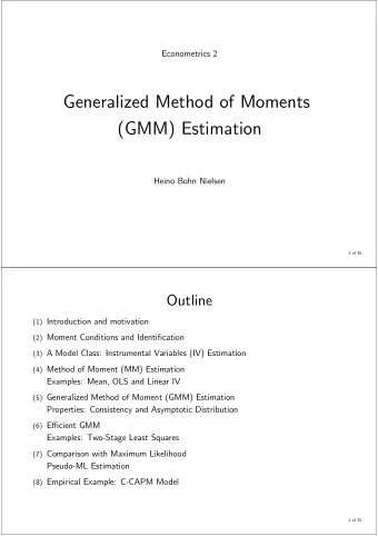
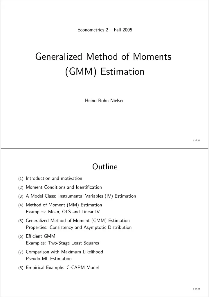
Econometrics 2 Fall 2005 Generalized Method of Moments (GMM) Estimation Heino Bohn Nielsen 1 of 32 Outline (1) Introduction and motivation (2) Moment Conditions and Identi fi cation (3) A Model Class: Instrumental Variables (IV) Estimation
Econometrics 2 — Fall 2005 Generalized Method of Moments (GMM) Estimation Heino Bohn Nielsen 1 of 32 Outline (1) Introduction and motivation (2) Moment Conditions and Identi fi cation (3) A Model Class: Instrumental Variables (IV) Estimation (4) Method of Moment (MM) Estimation Examples: Mean, OLS and Linear IV (5) Generalized Method of Moment (GMM) Estimation Properties: Consistency and Asymptotic Distribution (6) E ffi cient GMM Examples: Two-Stage Least Squares (7) Comparison with Maximum Likelihood Pseudo-ML Estimation (8) Empirical Example: C-CAPM Model 2 of 32
Introduction Generalized method of moments (GMM) is a general estimation principle. Estimators are derived from so-called moment conditions. Three main motivations: (1) Many estimators can be seen as special cases of GMM. Unifying framework for comparison. (2) Maximum likelihood estimators have the smallest variance in the class of consistent and asymptotically normal estimators. But: We need a full description of the DGP and correct speci fi cation. GMM is an alternative based on minimal assumptions. (3) GMM estimation is often possible where a likelihood analysis is extremely di ffi cult. We only need a partial speci fi cation of the model. Models for rational expectations. 3 of 32 Moment Conditions and Identi fi cation • A moment condition is a statement involving the data and the parameters: g ( θ 0 ) = E [ f ( w t , z t , θ 0 )] = 0 . ( ∗ ) where θ is a K × 1 vector of parameters; f ( · ) is an R dimensional vector of (non- linear) functions; w t contains model variables; and z t contains instruments. • If we knew the expectation then we could solve the equations in ( ∗ ) to fi nd θ 0 . • If there is a unique solution, so that E [ f ( w t , z t , θ )] = 0 θ = θ 0 , if and only if then we say that the system is identi fi ed. • Identi fi cation is essential for doing econometrics. Two ideas: (1) Is the model constructed so that θ 0 is unique (identi fi cation). (2) Are the data informative enough to determine θ 0 (empirical identi fi cation). 4 of 32
Instrumental Variables Estimation • In many applications, the moment condition has the speci fi c form: f ( w t , z t , θ ) = u ( w t , θ ) · z t , |{z} | {z } ( R × 1) (1 × 1) where the R instruments in z t are multiplied by the disturbance term, u ( w t , θ ) . • You can think of u ( w t , θ ) as the equivalent of an error term. The moment condition becomes g ( θ 0 ) = E [ u ( w t , θ 0 ) · z t ] = 0 , stating that the instruments are uncorrelated with the error term of the model. • This class of estimators is referred to as instrumental variables estimators. The function u ( w t , θ ) may be linear or non-linear in θ . 5 of 32 Example: Moment Condition From RE • Consider a monetary policy rule, where the interest rate depends on expected future in fl ation: r t = β · E [ π t +1 | I t ] + � t . Noting that x t +1 = E [ x t +1 | I t ] + v t , where v t is the expectation error, we can write the model as r t = β · E [ π t +1 | I t ] + � t = β · x t +1 + ( � t − β · v t ) = β · x t +1 + u t . • Under rational expectations, the expectation error, v t , should be orthogonal to the information set, I t , and for z t ∈ I t we have the moment condition E [ u t · z t ] = E [( r t − β · x t +1 ) · z t ] = 0 . This is enough to identify β . 6 of 32
Method of Moments (MM) Estimator • For a given sample, w t and z t ( t = 1 , 2 , ..., T ) , we cannot calculate the expectation. We replace with sample averages to obtain the analogous sample moments: X T g T ( θ ) = 1 f ( w t , z t , θ ) . T t =1 We can derive an estimator, b θ MM , as the solution to g T ( b θ MM ) = 0 . • To fi nd an estimator, we need at least as many equations as we have parameters. The order condition for identi fi cation is R ≥ K . — R = K is called exact identi fi cation. The estimator is denoted the method of moments estimator, b θ MM . — R > K is called over-identi fi cation. The estimator is denoted the generalized method of moments estimator, b θ GMM . 7 of 32 Example: MM Estimator of the Mean • Assume that y t is random variable drawn from a population with expectation µ 0 . We have a single moment condition: g ( µ 0 ) = E [ f ( y t , µ 0 )] = E [ y t − µ 0 ] = 0 , where f ( y t , µ 0 ) = y t − µ 0 . • For a sample, y 1 , y 2 , ..., y T , we state the corresponding sample moment conditions: X T µ ) = 1 g T ( b ( y t − b µ ) = 0 . T t =1 The MM estimator of the mean µ 0 is the solution, i.e. X T µ MM = 1 b y t , T t =1 which is the sample average. 8 of 32
Example: OLS as a MM Estimator • Consider the linear regression model of y t on x t ( K × 1 ): y t = x 0 t β 0 + � t . ( ∗∗ ) Assume that ( ∗∗ ) represents the conditional expectation: E [ y t | x t ] = x 0 t β 0 so that E [ � t | x t ] = 0 . • That implies the K unconditional moment conditions g ( β 0 ) = E [ x t � t ] = E [ x t ( y t − x 0 t β 0 )] = 0 , which we recognize as the minimal assumption for consistency of the OLS estimator. 9 of 32 • We de fi ne the corresponding sample moment conditions as ³ ´ T T T X X X β ) = 1 = 1 x t y t − 1 g T ( b t b t b y t − x 0 x t x 0 x t β β = 0 . T T T t =1 t =1 t =1 And the MM estimator is derived as the unique solution: Ã T ! − 1 X X T b x t x 0 β MM = x t y t , t t =1 t =1 provided that P T t =1 x t x 0 t is non-singular. • Method of moments is one way to motivate the OLS estimator. Highlights the minimal (or identifying) assumptions for OLS. 10 of 32
Example: Under-Identi fi cation • Consider again a regression model y t = x 0 t β 0 + � t = x 0 1 t γ 0 + x 0 2 t δ 0 + � t . • Assume that the K 1 variables in x 1 t are predetermined, while the K 2 = K − K 1 variables in x 2 t are endogenous. That implies E [ x 1 t � t ] = 0 ( K 1 × 1) ( † ) E [ x 2 t � t ] 6 = 0 ( K 2 × 1) . ( †† ) 0 , δ 0 • We have K parameters in β 0 = ( γ 0 0 ) 0 , but only K 1 < K moment conditions (i.e. K 1 equations to determine K unknowns). The parameters are not identi fi ed and cannot be estimated consistently. 11 of 32 Example: Simple IV Estimator • Assume K 2 new variables, z 2 t , that are correlated with x 2 t but uncorrelated with � t : E [ z 2 t � t ] = 0 . ( ††† ) The K 2 moment conditions in ( ††† ) can replace ( †† ). To simplify notation, we de fi ne µ ¶ µ ¶ x 1 t x 1 t x t = and z t = . x 2 t z 2 t ( K × 1) ( K × 1) x t are model variables, z 2 t are new instruments, and z t are instruments. We say that x 1 t are instruments for themselves. • Using ( † ) and ( ††† ) we have K moment conditions: µ ¶ E [ x 1 t � t ] = E [ z t � t ] = E [ z t ( y t − x 0 g ( β 0 ) = t β 0 )] = 0 , E [ z 2 t � t ] which are su ffi cient to identify the K parameters in β . 12 of 32
• The corresponding sample moment conditions are given by ³ ´ X T β ) = 1 g T ( b t b y t − x 0 z t β = 0 . T t =1 • The method of moments estimator is the unique solution: Ã T ! − 1 X X T b z t x 0 β MM = z t y t , t t =1 t =1 provided that P T t =1 z t x 0 t is non-singular. • Note the following: (1) We need the instruments to identify the parameters. (2) The MM estimator coincides with the simple IV estimator. (3) The procedure only works with K 2 instruments (i.e. R = K ). (4) Non-singularity of P T t =1 z t x 0 t requires relevant instruments. 13 of 32 Generalized Method of Moments Estimation • The case R > K is called over-identi fi cation. More equations than parameters and no solution to g T ( θ ) = 0 in general. • Instead we minimize the distance from g T ( θ ) to zero. The distance is measured by the quadratic form Q T ( θ ) = g T ( θ ) 0 W T g T ( θ ) , where W T is an R × R symmetric and positive de fi nite weight matrix. • The GMM estimator depends on the weight matrix: b { g T ( θ ) 0 W T g T ( θ ) } . θ GMM ( W T ) = arg min θ 14 of 32
Distances and Weight Matrices • Consider a simple example with 2 moment conditions µ ¶ g a g T ( θ ) = , g b where the dependence of T and θ is suppressed. • First consider a simple weight matrix, W T = I 2 : ¢ µ ¶ µ ¶ ¡ g a g b 1 0 g a Q T ( θ ) = g T ( θ ) 0 W T g T ( θ ) = = g 2 a + g 2 b , 0 1 g b which is the square of the simple distance from g T ( θ ) to zero. Here the coordinates are equally important. • Alternatively, look at a di ff erent weight matrix: ¢ µ ¶ µ ¶ ¡ g a g b 2 0 g a Q T ( θ ) = g T ( θ ) 0 W T g T ( θ ) = = 2 · g 2 a + g 2 b , 0 1 g b which attaches more weight to the fi rst coordinate in the distance. 15 of 32 Consistency: Why Does it Work? • Assume that a law of large numbers (LLN) applies to f ( w t , z t , θ ) , i.e. X T T − 1 f ( w t , z t , θ ) → E [ f ( w t , z t , θ )] for T → ∞ . t =1 That requires IID or stationarity and weak dependence. • If the moment conditions are correct, g ( θ 0 ) = 0 , then GMM is consistent, b θ GMM ( W T ) → θ 0 as T → ∞ , for any W T positive de fi nite. • Intuition: If a LLN applies, then g T ( θ ) converges to g ( θ ) . Since b θ GMM ( W T ) minimizes the distance from g T ( θ ) to zero, it will be a consistent estimator of the solution to g ( θ 0 ) = 0 . • The weight matrix, W T , has to be positive de fi nite, so that we put a positive and non-zero weight on all moment conditions. 16 of 32
Recommend
More recommend
Explore More Topics
Stay informed with curated content and fresh updates.
