Generalized Method of Moments (GMM) Estimation Heino Bohn Nielsen - PDF document

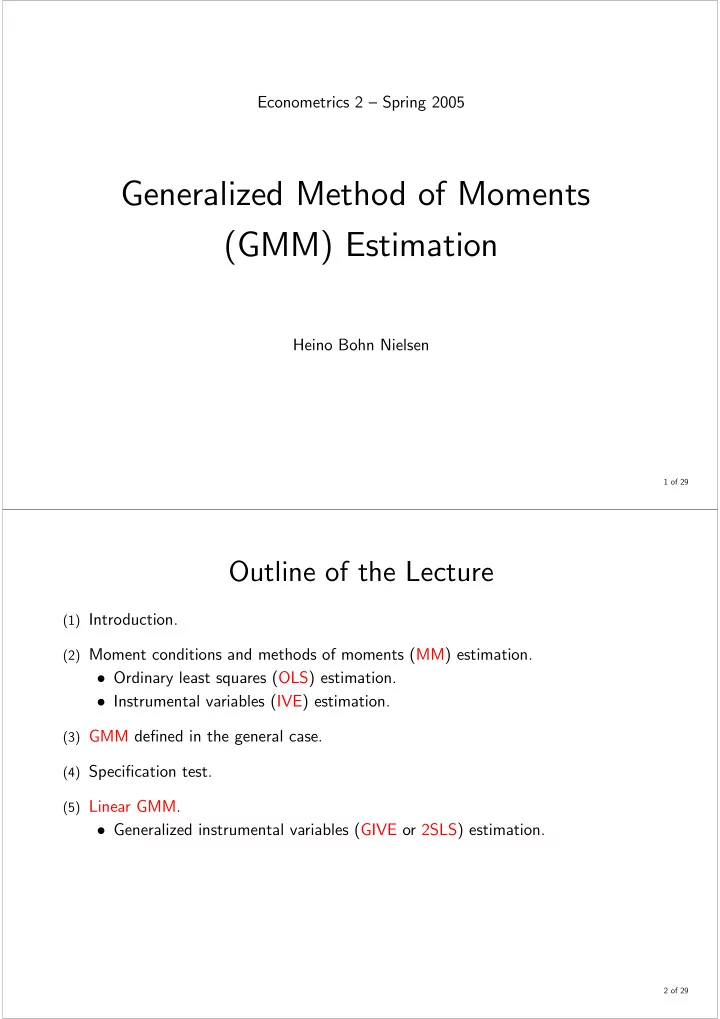
Econometrics 2 — Spring 2005 Generalized Method of Moments (GMM) Estimation Heino Bohn Nielsen 1 of 29 Outline of the Lecture (1) Introduction. (2) Moment conditions and methods of moments (MM) estimation. • Ordinary least squares (OLS) estimation. • Instrumental variables (IVE) estimation. (3) GMM de fi ned in the general case. (4) Speci fi cation test. (5) Linear GMM. • Generalized instrumental variables (GIVE or 2SLS) estimation. 2 of 29

Idea of GMM Estimation under weak assumptions; based on so-called moment conditions. Moment conditions are statements involving the data and the parameters. Arise naturally in many contexts. For example: (A) In a regression model, y t = x 0 t β + � t , we might think that E [ y t | x t ] = x 0 t β . This implies the moment condition E [ x t � t ] = E [ x t ( y t − x 0 t β )] = 0 . (B) Consider the economic relation y t = β · E [ x t +1 | I t ] + � t = β · x t +1 + ( β · ( E [ x t +1 | I t ] − x t +1 ) + � t ) | {z } u t Under rational expectations, the expectation error, E [ x t +1 | I t ] − x t +1 , should be orthogonal to the information set, I t , and for z t ∈ I t we have the moment condition E [ z t u t ] = 0 . 3 of 29 Properties of GMM GMM is a large sample estimator. Desirable properties as T → ∞ . • Consistent under weak assumptions. No distributional assumptions like in maximum likelihood (ML) estimation. • Asymptotically e ffi cient in the class of models that uses the same amount of infor- mation. • Many estimators are special cases of GMM. Unifying framework for comparing estimators. • GMM is a nonlinear procedure. We do not need a regression setup E [ y t ] = h ( x t ; β ) . We can have E [ f ( y t , x t ; β )] = 0 . 4 of 29

Moment Conditions and MM Estimation • Consider a variable y t with some (possibly unknown) distribution. Assume that the mean µ = E [ y t ] exists. We want to estimate µ . • We could state the population moment condition: E [ y t − µ ] = 0 , or E [ f ( y t , µ )] = 0 , where f ( y t , µ ) = y t − µ. • The parameter µ is identi fi ed by the condition if there is a unique solution, in the sense E [ f ( y t , µ )] = 0 only if µ = µ 0 . 5 of 29 • We cannot calculate E [ f ( y t , µ )] from an observed sample, y 1 , y 2 , ..., y t , ..., y T . De fi ne the sample moment condition as T T X X g T ( µ ) = 1 f ( y t , µ ) = 1 ( y t − µ ) = 0 . ( ∗ ) T T t =1 t =1 • By Law of Large Numbers, sample moments converge to population moments, g T ( µ ) → E [ f ( y t , µ )] T → ∞ . ( ∗∗ ) for The method of moments estimator, b µ MM , is the solution to ( ∗ ), i.e. X T µ MM = 1 b y t . T t =1 The sample average can be seen as a MM estimator. • MM estimator is consistent. Under weak regularity conditions ( ∗∗ ) implies b µ MM → µ 0 . 6 of 29

OLS as a MM Estimator • Consider the regression model with K explanatory variables y t = x 0 t β + � t . Assume no-contemporaneous-correlation (minimum for consistency of OLS): E [ x t � t ] = E [ x t ( y t − x 0 t β )] = ( K × 1) . 0 K moment conditions for the K parameters in β . • De fi ne the sample moment conditions X T g T ( β ) = 1 t β )) = 1 T X 0 ( Y − Xβ ) = ( x t ( y t − x 0 ( K × 1) . 0 T t =1 The MM estimator is given by the solution à T ! − 1 X X T b x t y t = ( X 0 X ) − 1 X 0 Y = b x t x 0 β MM = β OLS . t t =1 t =1 7 of 29 Instrumental Variables as a MM Estimator • Consider the regression model y t = x 0 1 t β 1 + x 2 t β 2 + � t , where the K − 1 variables in x 1 t are predetermined and x 2 t is endogenous: E [ x 1 t � t ] = 0 ( K − 1) × 1 E [ x 2 t � t ] 6 = 0 . ( # ) OLS is inconsistent! • Assume there exists a variable, z 2 t , such that corr ( x 2 t , z 2 t ) 6 = 0 E [ z 2 t � t ] = 0 (1 × 1) ( ## ) The new moment condition ( ## ) can replace ( # ). 8 of 29

• De fi ne µ ¶ µ ¶ x 1 t x 1 t K × 1 = x t and K × 1 = z t . x 2 t z 2 t z t are called instruments. z 2 t is the new instrument, The predetermined variables, x 1 t , are instruments for themselves. • The K population moment conditions are E [ z t � t ] = E [ z t ( y t − x 0 t β )] = ( K × 1) . 0 The K corresponding sample moment conditions are X T g T ( β ) = 1 t β )) = 1 T Z 0 ( Y − Xβ ) = ( z t ( y t − x 0 ( K × 1) . 0 T t =1 The MM estimator is given by the unique solution à T ! − 1 X X T b − 1 Z 0 Y = b z t x 0 z t y t = ( Z 0 X ) β MM = β IV . t | {z } t =1 t =1 ( K × K ) 9 of 29 Where do Instruments Come From? • Consider the two simple equations c t = β 10 + β 11 y t + β 12 w t + � 1 t y t = β 20 + β 21 c t + + β 22 w t + β 23 r t + β 24 τ t + � 2 t Say that we are only interested in the fi rst equation. • Assume that w t is predetermined. If β 21 6 = 0 , then y t is endogenous and E [ y t � 1 t ] 6 = 0 . • In this setup r t and τ t are possible instruments for y t . We need β 23 and β 24 di ff erent from zero and E [( r t , τ t ) � 1 t ] = 0 . • In dynamic models we can often use lagged values as instruments. Unfortunately, often poor... • Note, that in this case we have more potential instruments than we have endogenous variables. This is adressed in GMM/GIVE. 10 of 29

The GMM Problem De fi ned t ) 0 be a vector of model variables and let z t be instruments. • Let w t = ( y t , x 0 Consider the R moment conditions E [ f ( w t , z t , θ )] = 0 . Here θ is a K × 1 vector and f ( · ) is a R dimensional vector function. • Consider the corresponding sample moment conditions T X g T ( θ ) = 1 f ( w t , z t , θ ) = 0 . T t =1 • When can the R sample moments be used to estimate the K parameters in θ ? 11 of 29 Order Condition R < K No unique solution to g T ( θ ) = 0 . The parameters are not identi fi ed. R = K Unique solution to g T ( θ ) = 0 . Exact identi fi cation. This is the MM estimator (OLS, IV). Note, that g T ( θ ) = 0 is potentially a non-linear problem–numerical solution. R > K More equations than parameters. Over-identi fi ed case. No solution in general ( Z 0 X is a R × K matrix). • Not optimal to drop moments! • Instead, choose θ to make g T ( θ ) as close as possible to zero. 12 of 29

GMM Estimation ( R > K ) • We want to make the R moments g T ( θ ) as close to zero as possible...how? • Assume we have a R × R symmetric and positive de fi nite weight matrix W T . Then we could de fi ne the quadratic form Q T ( θ ) = g T ( θ ) 0 W T g T ( θ ) (1 × 1) . The GMM estimator is de fi ned as the vector that minimizes Q T ( θ ) , i.e. n o b g T ( b θ ) 0 W T g T ( b θ GMM ( W T ) = arg min θ ) . b θ • The matrix W T tells how much weight to put on each moment condition. Di ff erent W T give di ff erent estimators, b θ GMM ( W T ) . GMM is consistent for any weight matrix, W T . What is the optimal choice of W T ? 13 of 29 Optimal GMM Estimation • The R sample moments g T ( θ ) are estimators of E [ f ( · )] ; and random variables. The law of large numbers implies: g T ( θ ) → E [ f ( · )] T → ∞ . for A central limit theorem implies: √ T · g T ( θ ) → N (0 , S ) , √ where S is the asymptotic variance of the moments, T · g T ( θ ) . • Intuitively, moments with little variance should have large weights. The optimal weight matrix for GMM is a matrix W opt such that T = W opt = S − 1 . W opt plim T T →∞ 14 of 29

• Without autocorrelation, a natural estimator b S of S is h √ i b S = V T · g T ( θ ) = T · V [ g T ( θ )] " # T X 1 = T · V f ( w t , z t , θ ) T t =1 X T 1 f ( w t , z t , θ ) f ( w t , z t , θ ) 0 . = T · t =1 This implies that à ! − 1 X T 1 S − 1 = = b W opt f ( w t , z t , θ ) f ( w t , z t , θ ) 0 . T T t =1 • Note, that W opt depends on θ in general. T 15 of 29 Estimation in Practice • Two-step (e ffi cient) GMM. (1) Choose some initial weight matrix. E.g. W [1] = I or W [1] = ( Z 0 Z ) − 1 . Find a (consistent) estimator b g T ( θ ) 0 W [1] g T ( θ ) . θ [1] = arg min θ Estimate the optimal weights, W opt T . (2) Find the optimal GMM estimate b g T ( θ ) 0 W opt θ GMM = arg min T g T ( θ ) . θ • Iterated GMM. Start with some initial weight matrix W [1] . (1) Find an estimate b θ [1] . (2) Find a new weight matrix, W opt [2] . Iterate between b θ [ · ] and W opt until convergence. [ · ] 16 of 29

Properties of Optimal GMM • The GMM estimator, b θ GMM ( W opt T ) , is asymptotically e ffi cient. Lowest variance in a class of models that uses same information. • The GMM estimator is asymptotically normal, i.e. ³ ´ √ b T · θ GMM − θ → N (0 , V ) , where ¡ ¢ − 1 = ¡ ¢ − 1 D 0 W opt D D 0 S − 1 D V = D = plim ∂g T ( θ ) ( R × K ) . ∂θ 0 — S measures the variance of the moments. The larger S the larger V . — D measures the sensitivity of the moments wrt. changes in θ . If this is large the parameter can be estimated precisely. • Little is known in fi nite samples. 17 of 29 Speci fi cation Test • If R > K , we have more moments than parameters. All moments have expectation zero. In a sense K moments are zero by estimating the parameters. Test if the additional R − K moments are close to zero. If not, some orthogonality condition is violated. • Remember, that √ T · g T ( θ ) → N (0 , S ) . This implies that if the weights are optimal, W opt → S − 1 , then T µ 1 ¶ − 1 = g T ( b g T ( b θ GMM ) 0 ξ T S θ GMM ) = T · g T ( b T g T ( b θ GMM ) 0 W opt θ GMM ) → χ 2 ( R − K ) . Hansen test for overidentifying restrictions. (J-test, Sargan test). A test for R − K overidentifying conditions. 18 of 29