Generalized method of moments estimation of linear dynamic panel - PowerPoint PPT Presentation
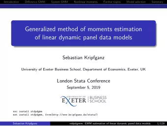
Introduction System GMM Postestimation Special features Summary Generalized method of moments estimation of linear dynamic panel data models Sebastian Kripfganz University of Exeter Business School, Department of Economics, Exeter, UK Stata
Introduction System GMM Postestimation Special features Summary Generalized method of moments estimation of linear dynamic panel data models Sebastian Kripfganz University of Exeter Business School, Department of Economics, Exeter, UK Stata Conference July 31, 2020 ssc install xtdpdgmm net install xtdpdgmm, from(http://www.kripfganz.de/stata/) Sebastian Kripfganz xtdpdgmm: GMM estimation of linear dynamic panel data models 1/38
Introduction System GMM Postestimation Special features Summary GMM estimation of linear dynamic panel data models Instrumental variables (IV) / generalized method of moments (GMM) estimation is the predominant estimation technique for panel data models with unobserved unit-specific heterogeneity and endogenous variables, in particular lagged dependent variables, when the time horizon is short. This presentation introduces the community-contributed xtdpdgmm Stata command. For a longer version of this talk with many additional details, see my 2019 London Stata Conference presentation: https://www.stata.com/meeting/uk19/slides/uk19_kripfganz.pdf Sebastian Kripfganz xtdpdgmm: GMM estimation of linear dynamic panel data models 2/38
Introduction System GMM Postestimation Special features Summary GMM estimation of linear dynamic panel data models Official Stata commands: xtdpd command for the Arellano and Bond (1991) difference GMM (diff-GMM) and the Arellano and Bover (1995) and Blundell and Bond (1998) system GMM (sys-GMM) estimation. xtabond command for diff-GMM estimation; xtdpd wrapper. xtdpdsys command for sys-GMM estimation; xtdpd wrapper. gmm command for GMM estimation (not just of dynamic panel data models). Community-contributed Stata commands: xtabond2 command by Roodman (2009) for diff-GMM and sys-GMM estimation. xtdpdgmm command for diff-GMM, sys-GMM, and GMM estimation with the Ahn and Schmidt (1995) nonlinear moment conditions. Sebastian Kripfganz xtdpdgmm: GMM estimation of linear dynamic panel data models 3/38
Introduction System GMM Postestimation Special features Summary Concerns about existing Stata commands Official Stata commands lack flexibility and suffer from bugs: Specification of time dummies i. timevar : collinearity checks in xtdpd (and therefore also xtabond and xtdpdsys ) lead to the omission of 1 time dummy too many. xtdpd and gmm yield incorrect estimates in some cases of unbalanced panel data sets. Option diffvars() of xtabond yields incorrect predictions. Community-contributed Stata command xtabond2 suffers from bugs as well: Incorrect estimates in some cases when forward-orthogonal deviations are combined with standard instruments. Incorrect estimates in some cases of unbalanced panel data sets. Incorrect degrees of freedom and p -values for the overidentification tests if some coefficients are shown as omitted (or empty ), a typical concern with time dummies. Sebastian Kripfganz xtdpdgmm: GMM estimation of linear dynamic panel data models 4/38
Introduction System GMM Postestimation Special features Summary Linear dynamic panel data model Linear dynamic panel data model: y it = λ y i , t − 1 + x ′ it β + α i + u it � �� � = e it with many cross-sectional units i = 1 , 2 , . . . , N and few time periods t = 1 , 2 , . . . , T . Further lags of y it and x it can be added as regressors. The regressors x it can be strictly exogenous, weakly exogenous (predetermined), or endogenous. The idiosyncratic error term u it shall be serially uncorrelated. The unobserved unit-specific heterogeneity α i can be correlated with the regressors x it . It is correlated by construction with the lagged dependent variable y i , t − 1 . Sebastian Kripfganz xtdpdgmm: GMM estimation of linear dynamic panel data models 5/38
Introduction System GMM Postestimation Special features Summary Model transformations supported by xtdpdgmm First-difference transformation (Anderson and Hsiao, 1981; Arellano and Bond, 1991), option model(difference) : ∆ y it = λ ∆ y i , t − 1 + ∆ x ′ it β + ∆ e it Forward-orthogonal deviations (Arellano and Bover, 1995), option model(fodev) : ∆ t y it = λ ˜ ˜ ∆ t y i , t − 1 + ˜ it β + ˜ ∆ t x ′ ∆ t e it � � � where ˜ T − t +1 1 � T − t ∆ t e it = . e it − s =0 e i , t + s T − t +1 T − t Deviations from within-group means, option model(mdev) : ∆ y it = λ ¨ ¨ ∆ y i , t − 1 + ¨ it β + ¨ ∆ x ′ ∆ e it � where ¨ T ∆ e it = T − 1 ( e it − ¯ e i ). Sebastian Kripfganz xtdpdgmm: GMM estimation of linear dynamic panel data models 6/38
Introduction System GMM Postestimation Special features Summary GMM-type instruments Stacked moment conditions (for the first-differenced model): � � ′ ∆ e i Z D = 0 E i where ∆ e i = (∆ e i 2 , ∆ e i 3 , . . . , ∆ e iT ) ′ , and Z D i = ( Z D yi , Z D xi ), with GMM-type instruments y i 0 0 0 0 0 0 t = 2 · · · · · · ← 0 y i 0 y i 1 0 0 0 t = 3 · · · · · · ← Z D yi = . . ... . . . . 0 0 0 y i 0 y i 1 y i , T − 2 t = T · · · · · · ← and similarly for Z D xi . Moment conditions for other model transformations are stacked likewise. Sebastian Kripfganz xtdpdgmm: GMM estimation of linear dynamic panel data models 7/38
Introduction System GMM Postestimation Special features Summary One-step diff-GMM estimation GMM-type instruments specified with the gmmiv() option, exemplarily for predetermined w and strictly exogenous k : . webuse abdata . xtdpdgmm L(0/1).n w k, model(diff) gmm(n, lag(2 .)) gmm(w, lag(1 .)) gmm(k, lag(. .)) nocons note: standard errors may not be valid Generalized method of moments estimation Fitting full model: Step 1 f(b) = .01960406 Group variable: id Number of obs = 891 Time variable: year Number of groups = 140 Moment conditions: linear = 126 Obs per group: min = 6 nonlinear = 0 avg = 6.364286 total = 126 max = 8 ------------------------------------------------------------------------------ n | Coef. Std. Err. z P>|z| [95% Conf. Interval] -------------+---------------------------------------------------------------- n | L1. | .4144164 .0341502 12.14 0.000 .3474833 .4813495 | w | -.8292293 .0588914 -14.08 0.000 -.9446543 -.7138042 k | .3929936 .0223829 17.56 0.000 .3491239 .4368634 ------------------------------------------------------------------------------ (Continued on next page) Sebastian Kripfganz xtdpdgmm: GMM estimation of linear dynamic panel data models 8/38
Introduction System GMM Postestimation Special features Summary One-step diff-GMM estimation Instruments corresponding to the linear moment conditions: 1, model(diff): 1978:L2.n 1979:L2.n 1980:L2.n 1981:L2.n 1982:L2.n 1983:L2.n 1984:L2.n 1979:L3.n 1980:L3.n 1981:L3.n 1982:L3.n 1983:L3.n 1984:L3.n 1980:L4.n 1981:L4.n 1982:L4.n 1983:L4.n 1984:L4.n 1981:L5.n 1982:L5.n 1983:L5.n 1984:L5.n 1982:L6.n 1983:L6.n 1984:L6.n 1983:L7.n 1984:L7.n 1984:L8.n 2, model(diff): 1978:L1.w 1979:L1.w 1980:L1.w 1981:L1.w 1982:L1.w 1983:L1.w 1984:L1.w 1978:L2.w 1979:L2.w 1980:L2.w 1981:L2.w 1982:L2.w 1983:L2.w 1984:L2.w 1979:L3.w 1980:L3.w 1981:L3.w 1982:L3.w 1983:L3.w 1984:L3.w 1980:L4.w 1981:L4.w 1982:L4.w 1983:L4.w 1984:L4.w 1981:L5.w 1982:L5.w 1983:L5.w 1984:L5.w 1982:L6.w 1983:L6.w 1984:L6.w 1983:L7.w 1984:L7.w 1984:L8.w 3, model(diff): 1978:F6.k 1978:F5.k 1979:F5.k 1978:F4.k 1979:F4.k 1980:F4.k 1978:F3.k 1979:F3.k 1980:F3.k 1981:F3.k 1978:F2.k 1979:F2.k 1980:F2.k 1981:F2.k 1982:F2.k 1978:F1.k 1979:F1.k 1980:F1.k 1981:F1.k 1982:F1.k 1983:F1.k 1978:k 1979:k 1980:k 1981:k 1982:k 1983:k 1984:k 1978:L1.k 1979:L1.k 1980:L1.k 1981:L1.k 1982:L1.k 1983:L1.k 1984:L1.k 1978:L2.k 1979:L2.k 1980:L2.k 1981:L2.k 1982:L2.k 1983:L2.k 1984:L2.k 1979:L3.k 1980:L3.k 1981:L3.k 1982:L3.k 1983:L3.k 1984:L3.k 1980:L4.k 1981:L4.k 1982:L4.k 1983:L4.k 1984:L4.k 1981:L5.k 1982:L5.k 1983:L5.k 1984:L5.k 1982:L6.k 1983:L6.k 1984:L6.k 1983:L7.k 1984:L7.k 1984:L8.k xtdpdgmm has the options nolog , noheader , notable , and nofootnote to suppress undesired output. Sebastian Kripfganz xtdpdgmm: GMM estimation of linear dynamic panel data models 9/38
Introduction System GMM Postestimation Special features Summary Too-many-instruments problem Too many instruments relative to the cross-sectional sample size can aggravate finite-sample biases in the coefficient and standard error estimates and potentially weakens specification tests (Roodman, 2009a). To reduce the number of instruments, two main approaches are typically used (Roodman, 2009a, 2009b; Kiviet, 2020): Curtailing: Limit the number of lags used as instruments, suboption lagrange() , e.g. y i , t − 2 , y i , t − 3 , . . . , y i , t − l . Collapsing: Use standard instruments instead of GMM-type instruments, suboption collapse or option iv() , e.g. y i 0 0 0 t = 2 · · · ← y i 1 y i 0 0 t = 3 · · · ← Z D yi = . . . . . ... . . . . . . . . . . t = T y i , T − 2 y i , T − 3 y i 0 · · · ← Sebastian Kripfganz xtdpdgmm: GMM estimation of linear dynamic panel data models 10/38
Recommend
More recommend
Explore More Topics
Stay informed with curated content and fresh updates.
