Probabilistic Methods for Complex Networks Lecture 6: Random - PowerPoint PPT Presentation

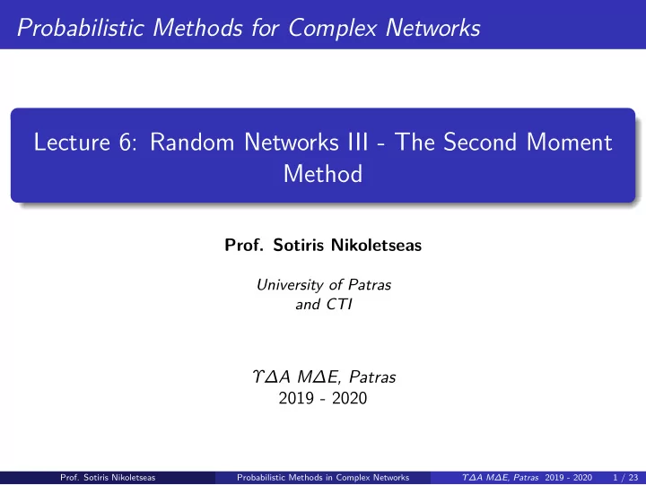
Probabilistic Methods for Complex Networks Lecture 6: Random Networks III - The Second Moment Method Prof. Sotiris Nikoletseas University of Patras and CTI ΥΔΑ ΜΔΕ, Patras 2019 - 2020 Prof. Sotiris Nikoletseas Probabilistic Methods in Complex Networks ΥΔΑ ΜΔΕ, Patras 2019 - 2020 1 / 23

Summary of this lecture v. ΥΔΑ ΜΔΕ, Patras 2019 - 2020 Probabilistic Methods in Complex Networks Prof. Sotiris Nikoletseas Example - Cliques of size 4 in random graphs. vi. variables. Alternative techniques of estimation of the variance of a sum of indicator Covariance The Second Moment iv. The Second Moment method iii. The Chebyshev Inequality ii. The Variance of a random variable i. 2 / 23

Variance Variance: ΥΔΑ ΜΔΕ, Patras 2019 - 2020 Probabilistic Methods in Complex Networks Prof. Sotiris Nikoletseas Standard deviation: 3 / 23 properties: is the most vital statistic of a r.v. beyond expectation. � ( X − E [ X ]) 2 � is defjned as V ar [ X ] = E V ar ( X ) = E [ X 2 ] − E 2 [ X ] V ar ( cX ) = c 2 V ar ( X ) , c constant X, Y independent ⇒ V ar [ X + Y ] = V ar [ X ] + V ar [ Y ] � V ar [ X ] ⇒ V ar [ X ] = σ 2 σ =

Chebyshev Inequality Theorem 1 (Chebyshev Inequality) ΥΔΑ ΜΔΕ, Patras 2019 - 2020 Probabilistic Methods in Complex Networks Prof. Sotiris Nikoletseas 4 / 23 Proof: Let X be a random variable with expected value µ . Then for any t > 0 : Pr [ | X − µ | ≥ t ] ≤ V ar [ X ] t 2 ( X − µ ) 2 ≥ t 2 � � Pr[ | X − µ | ≥ t ] = Pr � ( X − µ ) 2 � E = V ar [ X ] ≤ t 2 t 2 Markov �

Chebyshev Inequality Alternative Proof: ΥΔΑ ΜΔΕ, Patras 2019 - 2020 Probabilistic Methods in Complex Networks Prof. Sotiris Nikoletseas 5 / 23 ( x − µ ) 2 Pr { X = x } � � ( X − µ ) 2 � V ar [ X ] = E = x ( x − µ ) 2 Pr { X = x } � ≥ | x − µ |≥ t t 2 Pr { X = x } � ≥ | x − µ |≥ t Pr { X = x } = t 2 Pr {| X − µ | ≥ t } � = t 2 | x − µ |≥ t ⇒ Pr {| X − µ | ≥ t } ≤ V ar [ X ] t 2 �

Chebyshev Inequality - application . ΥΔΑ ΜΔΕ, Patras 2019 - 2020 Probabilistic Methods in Complex Networks Prof. Sotiris Nikoletseas A small variance implies high concentration. around its mean. In other words, this inequality bounds the concentration of a random variable 6 / 23 . . if t = σ then Pr[ | X − µ | ≥ σ ] ≤ σ 2 σ 2 = 1 (trivial bound) σ 2 (2 σ ) 2 = 1 if t = 2 σ then Pr[ | X − µ | ≥ 2 σ ] ≤ 4 σ 2 1 if t = kσ then Pr[ | X − µ | ≥ kσ ] ≤ ( kσ ) 2 = k 2

The Second Moment Method Theorem 2 ΥΔΑ ΜΔΕ, Patras 2019 - 2020 Probabilistic Methods in Complex Networks Prof. Sotiris Nikoletseas terms of the mean. So, we need to estimate the variance. Actually, we need to properly bound it in 7 / 23 or Proof : Since For any random variable X it holds that: if E [ X ] → ∞ and V ar [ X ] = o ( E 2 [ X ]) then Pr { X = 0 } → 0 � X ≥ 2 E [ X ] | X − E [ X ] | ≥ E [ X ] ⇒ X ≤ 0 V ar [ X ] Pr { X = 0 } ≤ Pr {| X − E [ X ] | ≥ E [ X ] } ≤ E 2 [ X ] t = E [ X ] if V ar [ X ] E 2 [ X ] → 0 ⇔ V ar [ X ] = o ( E 2 [ X ]) then Pr { X = 0 } → 0 �

Covariance Covariance Let X and Y be random variables. Then Remark: Covariance is a measure of association between two random variables. Prof. Sotiris Nikoletseas Probabilistic Methods in Complex Networks ΥΔΑ ΜΔΕ, Patras 2019 - 2020 8 / 23 Cov ( X, Y ) = E [ XY ] − E [ X ] · E [ Y ] Cov ( X, X ) = V ar [ X ] if X, Y are independent r.v. then Cov ( X, Y ) = 0 | Cov ( X, Y ) | ↑ ⇒ stochastic dependence of X, Y ↑

Covariance Variance - Covariance Theorem 3 Prof. Sotiris Nikoletseas Probabilistic Methods in Complex Networks ΥΔΑ ΜΔΕ, Patras 2019 - 2020 9 / 23 Consider a sum of n random variables X = X 1 + X 2 + · · · + X n . It holds that: � V ar [ X ] = Cov ( X i , X j ) 1 ≤ i,j ≤ n Remark: The sum is over ordered pairs, i.e. we take both Cov ( X i , X j ) and Cov ( X j , X i ) .

Proof of theorem 3 Prof. Sotiris Nikoletseas ΥΔΑ ΜΔΕ, Patras 2019 - 2020 Probabilistic Methods in Complex Networks 10 / 23 The proof is by induction on n . We show the case n = 2 : � Cov ( X i , X j ) = Cov ( X 1 , X 1 ) + Cov ( X 1 , X 2 )+ 1 ≤ i,j ≤ 2 + Cov ( X 2 , X 1 ) + Cov ( X 2 , X 2 ) = E [ X 2 1 ] − E 2 [ X 1 ] + E [ X 1 X 2 ] − E [ X 1 ] E [ X 2 ] + E [ X 2 X 1 ] − E [ X 2 ] E [ X 1 ]+ + E [ X 2 2 ] − E 2 [ X 2 ] = = E [ X 2 1 ] + E [ X 2 2 ] + 2 E [ X 1 X 2 ] − ( E 2 [ X 1 ] + E 2 [ X 2 ] + 2 E [ X 1 ] E [ X 2 ]) = − ( E [ X 1 ] + E [ X 2 ]) 2 X 2 1 + X 2 � � = E 2 + 2 X 1 X 2 − E 2 [( X 1 + X 2 )] = ( X 1 + X 2 ) 2 � � = E = V ar [ X 1 + X 2 ]

Covariance It holds that: ΥΔΑ ΜΔΕ, Patras 2019 - 2020 Probabilistic Methods in Complex Networks Prof. Sotiris Nikoletseas Proof: An upper bound of the sum of indicator r.v. 11 / 23 Theorem 4 Let X i 1 ≤ i ≤ n be indicator random variables. � 1 p i X i = 0 1 − p i Let X be their sum: X = X 1 + X 2 + · · · + X n . � V ar [ X ] ≤ E [ X ] + Cov ( X i , X j ) 1 ≤ i � = j ≤ n V ar [ X ] = � 1 ≤ i,j ≤ n Cov ( X i , X j ) ( X i ) 2 � − E 2 [ X i ] = V ar [ X i ] � Cov ( X i , X i ) = E [ X i X i ] − E [ X i ] E [ X i ] = E

Covariance Proof of theorem 4 ΥΔΑ ΜΔΕ, Patras 2019 - 2020 Probabilistic Methods in Complex Networks Prof. Sotiris Nikoletseas 12 / 23 V ar [ X i ] = (1 − p i ) 2 · p i + (0 − p i ) 2 · (1 − p i ) = p i (1 − p i ) ≤ p i = E [ X i ] � � V ar [ X ] = Cov ( X i , X i ) + Cov ( X i , X j ) 1 ≤ i ≤ n 1 ≤ i � = j ≤ n � � = V ar [ X i ] + Cov ( X i , X j ) 1 ≤ i ≤ n 1 ≤ i � = j ≤ n � � ≤ E [ X i ] + Cov ( X i , X j ) 1 ≤ i ≤ n 1 ≤ i � = j ≤ n � = E [ X ] + Cov ( X i , X j ) 1 ≤ i � = j ≤ n �

Bounding the Variance The sum is over ordered pairs. ΥΔΑ ΜΔΕ, Patras 2019 - 2020 Probabilistic Methods in Complex Networks Prof. Sotiris Nikoletseas 13 / 23 We defjne Suppose that X = X 1 + X 2 + · · · + X n where X i is the indicator r.v. for event A i . For indices i, j we defjne the operator ∼ and write i ∼ j if i � = j and the events A i and A j are not independent. (non-trivial dependence) � ∆ = Pr { A i ∧ A j } i ∼ j Cov ( X i , X j ) = E [ X i X j ] − E [ X i ] E [ X j ] ≤ E [ X i X j ] = Pr { A i ∧ A j } ⇒ V ar [ X ] ≤ E [ X ] + ∆

The Basic Theorem Theorem 5 ΥΔΑ ΜΔΕ, Patras 2019 - 2020 Probabilistic Methods in Complex Networks Prof. Sotiris Nikoletseas 14 / 23 Proof: If E [ X ] → ∞ and ∆ = o ( E 2 [ X ]) then Pr { X = 0 } → 0 Pr { X = 0 } ≤ V ar [ X ] E 2 [ X ] ≤ E [ X ] + ∆ 1 ∆ = E [ X ] + E 2 [ X ] → 0 E 2 [ X ] �

A variation (I) Symmetric events: In other words, the conditional probability of a pair of events is independent of the “order” of conditioning. Symmetry applies in almost all graphotheoretical properties because of symmetry of corresponding subgraphs which are set of vertices (i.e. the conditioning afgects the intersection and depends on its size). Prof. Sotiris Nikoletseas Probabilistic Methods in Complex Networks ΥΔΑ ΜΔΕ, Patras 2019 - 2020 15 / 23 Events A i and A j are symmetric if and only if Pr { X i | X j = 1 } = Pr { X j | X i = 1 }

A variation (II) Proof: ΥΔΑ ΜΔΕ, Patras 2019 - 2020 Probabilistic Methods in Complex Networks Prof. Sotiris Nikoletseas We defjne 16 / 23 ∆ ∗ = � Pr { A j | A i } j ∼ i Lemma: ∆ = ∆ ∗ · E [ X ] � � ∆ = Pr { A i ∧ A j } = Pr { A i } Pr { A j | A i } i ∼ j i ∼ j � � = Pr { A i } Pr { A j | A i } i j ∼ i � � = Pr { A i } Pr { A j | A i } i j ∼ i = ∆ ∗ · � Pr { A i } i ⇒ ∆ = ∆ ∗ · E [ X ] �

The basic theorem of the variation Change of previous theorem’s condition: Theorem 6 Prof. Sotiris Nikoletseas Probabilistic Methods in Complex Networks ΥΔΑ ΜΔΕ, Patras 2019 - 2020 17 / 23 ∆ = o ( E 2 [ X ]) ⇔ ∆ ∗ · E [ X ] = o ( E 2 [ X ]) ⇔ ∆ ∗ = o ( E [ X ]) If E [ X ] → ∞ and ∆ ∗ = o ( E [ X ]) then Pr { X = 0 } → 0

18 / 23 Defjnition 7 ΥΔΑ ΜΔΕ, Patras 2019 - 2020 Probabilistic Methods in Complex Networks Prof. Sotiris Nikoletseas hamiltonicity: connectivity: giant component: Typical thresholds: Threshold functions in G n,p p o = p o ( n ) is a threshold of property A ifg p >> p o ⇒ Pr { G n,p has the property A } → 1 p << p o ⇒ Pr { G n,p has the property A } → 0 c n (c constant) c log n n c log n n

Example S is clique ΥΔΑ ΜΔΕ, Patras 2019 - 2020 Probabilistic Methods in Complex Networks Prof. Sotiris Nikoletseas otherwise 19 / 23 Proof: Let S be any fjxed set of 4 vertices. Theorem 8 Existence of complete subgraph of size 4 in G n,p Let A be the property of existence of K 4 cliques in G n,p . The threshold function for A is p o ( n ) = n − 2 / 3 . Defjne r.v. X that counts the number of cliques of size 4. X = � S, | S | =4 X S where X S is an indicator variable: � 1 X S = 0 E [ X S ] = p 6

Proof of theorem 8 By Linearity of expectation ΥΔΑ ΜΔΕ, Patras 2019 - 2020 Probabilistic Methods in Complex Networks Prof. Sotiris Nikoletseas 20 / 23   � n � p 6 ∼ n 4 p 6  � �  = E [ X ] = E X S E [ X S ] = 4 S, | S | =4 S, | S | =4 E [ X ] = n 4 p 6 << 1 ⇔ p << n − 2 / 3 If p << n − 2 / 3 ⇒ E [ X ] → 0 ⇒ non-existence w.h.p. Also, clearly p >> n − 2 / 3 ⇒ E [ X ] → ∞ .