A Course in Applied Econometrics Outline Lecture 16 1. - PowerPoint PPT Presentation
A Course in Applied Econometrics Outline Lecture 16 1. Introduction 2. Generalized Method of Moments Estimation Generalized Method of Moments and Empirical Likelihood 3. Empirical Likelihood 4. Computational Issues Guido Imbens 5. A
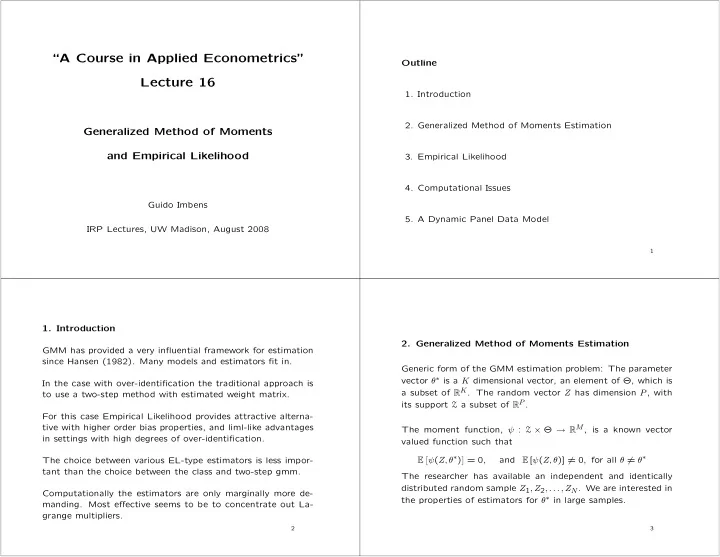
“A Course in Applied Econometrics” Outline Lecture 16 1. Introduction 2. Generalized Method of Moments Estimation Generalized Method of Moments and Empirical Likelihood 3. Empirical Likelihood 4. Computational Issues Guido Imbens 5. A Dynamic Panel Data Model IRP Lectures, UW Madison, August 2008 1 1. Introduction 2. Generalized Method of Moments Estimation GMM has provided a very influential framework for estimation since Hansen (1982). Many models and estimators fit in. Generic form of the GMM estimation problem: The parameter vector θ ∗ is a K dimensional vector, an element of Θ, which is In the case with over-identification the traditional approach is a subset of R K . The random vector Z has dimension P , with to use a two-step method with estimated weight matrix. its support Z a subset of R P . For this case Empirical Likelihood provides attractive alterna- tive with higher order bias properties, and liml-like advantages The moment function, ψ : Z × Θ → R M , is a known vector in settings with high degrees of over-identification. valued function such that � = 0 , � ψ ( Z, θ ∗ ) and E [ ψ ( Z, θ )] � = 0 , for all θ � = θ ∗ The choice between various EL-type estimators is less impor- E tant than the choice between the class and two-step gmm. The researcher has available an independent and identically distributed random sample Z 1 , Z 2 , . . . , Z N . We are interested in Computationally the estimators are only marginally more de- the properties of estimators for θ ∗ in large samples. manding. Most effective seems to be to concentrate out La- grange multipliers. 2 3
Example I: Maximum Likelihood Example II: Linear Instrumental Variables If one specifies the conditional distribution of a variable Y given another variable X as f Y | X ( y | x, θ ), the score function satisfies Suppose one has a linear model these conditions for the moment function: Y = X ′ θ ∗ + ε, ψ ( Y, X, θ ) = ∂ ln f ∂θ ( Y | X, θ ) . with a vector of instruments Z . In that case the moment By standard likelihood theory the score function has expecta- function is tion zero only at the true value of the parameter. ψ ( Y, X, Z, θ ) = Z ′ · ( Y − X ′ θ ) . The validity of Z as an instrument, together with a rank condi- Interpreting maximum likelihood estimators as generalized method tion implies that θ ∗ is the unique solution to E [ ψ ( Y, X, Z, θ )] = of moments estimators suggests a way of deriving the covari- 0. ance matrix under misspecification (e.g., White, 1982), as well as an interpretation of the estimand in that case. 4 5 One can construct moment functions by differencing and using lags as instruments, as in Arellano and Bond (1991), and Ahn Example III: A Dynamic Panel Data Model and Schmidt, (1995): ⎛ Y it − 2 ⎞ Consider the following panel data model with fixed effects: Y it − 3 � � ⎜ ⎟ ψ 1 t ( Y i 1 , . . . , Y iT , θ ) = ⎠ · ( Y it − Y it − 1 − θ · ( Y it − 1 − Y it − 2 ) . ⎜ . ⎟ . . Y it = η i + θ · Y it − 1 + ε it , ⎜ ⎟ ⎝ Y i 1 where ε it has mean zero given { Y it − 1 , Y it − 2 , . . . } . We have ob- This leads to t − 2 moment functions for each value of t = servations Y it for t = 1 , . . . , T and i = 1 , . . . , N , with N large 3 , . . . , T , leading to a total of ( T − 1) · ( T − 2) / 2 moments, with relative to T . only a single parameter ( θ ). This is a stylized version of the type of panel data models In addition, under the assumption that the initial condition is studied in Keane and Runkle (1992), Chamberlain (1992), and drawn from the stationary long-run distribution, the following Blundell and Bond (1998). This specific model has previously additional T − 2 moments are valid: been studied by Bond, Bowsher, and Windmeijer (2001). ψ 2 t ( Y i 1 , . . . , Y iT , θ ) = ( Y it − 1 − Y it − 2 ) · ( Y it − θ · Y it − 1 ) . 6 7
GMM: Estimation GMM: Large Sample Properties Under regularity conditions the minimand ˆ In the just-identified case where M , the dimension of ψ , and θ gmm has the follow- K , the dimension of θ are identical, one can generally estimate ing large sample properties: θ ∗ by solving p → θ ∗ , ˆ θ gmm − N 0 = 1 √ � ψ ( Z i , ˆ θ gmm ) . (1) d θ gmm − θ ∗ ) → N (0 , (Γ ′ C Γ) − 1 Γ ′ C ∆ C Γ(Γ ′ C Γ) − 1 ) , N (ˆ − N i =1 where Under regularity conditions solutions will be unique in large � ∂ samples and consistent for θ ∗ . If M > K there is in general � � ψ ( Z i , θ ∗ ) ψ ( Z i , θ ∗ ) ′ � ∂θ ′ ψ ( Z i , θ ∗ ) ∆ = E and Γ = E . there will be no solution to (1). In the just–identified case with the number of parameters K Hansen’s solution was to minimize the quadratic form equal to the number of moments M , the choice of weight � N � N matrix C is immaterial. � ′ � Q C,N ( θ ) = 1 � � ψ ( z i , θ ) · C · ψ ( z i , θ ) , N In that case Γ is a square matrix, and because it is full rank i =1 i =1 for some positive definite M × M symmetric matrix C (which by assumption, Γ is invertible and the asymptotic covariance matrix reduces to (Γ ′ ∆ − 1 Γ) − 1 , irrespective of the choice of C . if M = K still leads to a ˆ θ that solves the equation (1). 8 9 This estimator is not feasible because ∆ − 1 is unknown. GMM: Optimal Weight Matrix The feasible solution is to obtain an initial consistent, but gen- erally inefficient, estimate of θ ∗ and then can estimate the In the overidentified case with M > K the choice of the weight optimal weight matrix as matrix C is important. � − 1 N � 1 ∆ − 1 = θ ) ′ ˆ � ψ ( z i , ˜ θ ) · ψ ( z i , ˜ . N i =1 The optimal choice for C in terms of minimizing the asymptotic In the second step one estimates θ ∗ by minimizing Q ˆ ∆ − 1 ,N ( θ ). variance is in this case the inverse of the covariance of the moments, ∆ − 1 . The resulting estimator ˆ θ gmm has the same first order asymp- totic distribution as the minimand of the quadratic form with Then: the true, rather than estimated, optimal weight matrix, Q ∆ − 1 ,N ( θ ). √ d θ gmm − θ ∗ ) → N (0 , (Γ ′ ∆ − 1 Γ) − 1 ) . N (ˆ − (2) Compare to TSLS having the same asymptotic distribution as estimator with optimal instrument. 10 11
GMM: Specification Testing Interpreting Over-identified GMM as a Just-identified Mo- ment Estimator If the number of moments exceeds the number of free param- eters, not all average moments can be set equal to zero, and One can also interpret the two–step estimator for over–identified their deviation from zero forms the basis of a test.Formally, GMM models as a just–identified GMM estimator with an aug- the test statistic is mented parameter vector. Fix an arbitrary M × M postitive definite matrix C . Then: ∆ ,N (ˆ T = Q ˆ θ gmm ) . ⎛ Λ − ∂ψ ⎞ ∂θ ′ ( x, β ) Under the null hypothesis that all moments have expectation Λ ′ Cψ ( x, β ) ⎜ ⎟ ⎜ ⎟ equal to zero at the true value of the parameter the distribution ⎜ ⎟ ∆ − ψ ( x, β ) ψ ( x, β ) ′ h ( x, δ ) = h ( x, θ, Γ , ∆ , β, Λ) = . (3) ⎜ ⎟ ⎜ ⎟ of the test statistic converges to a chi-squared distribution with Γ − ∂ψ ⎜ ⎟ ∂θ ′ ( x, θ ) ⎜ ⎟ degrees of freedom equal to the number of over-identifying ⎝ ⎠ Γ ′ ∆ − 1 ψ ( x, θ ) restrictions, M − K . 12 13 Efficiency This interpretation emphasizes that results for just–identified Chamberlain (1987) demonstrated that Hansen’s (1982) esti- GMM estimators such as the validity of the bootstrap can di- mator is efficient, not just in the class of estimators based on rectly be translated into results for over–identified GMM esti- minimizing the quadratic form Q N,C ( θ ), but in the larger class mators. of semiparametric estimators exploiting the full set of moment conditions. For example, one can use the just-identified representation to find the covariance matrix for the over–identified GMM esti- Chamberlain assumes that the data are discrete with finite sup- mator that is robust against misspecification: the appropriate port { λ 1 , . . . , λ L } , and unknown probabilities π 1 , . . . , π L . The submatrix of parameters of interest are then implicitly defined as functions �� − 1 �� − 1 � ∂h � ∂h � � of these points of support and probabilities. With only the ∂δ ( X, δ ∗ ) E [ h ( Z, δ ∗ ) h ( Z, δ ∗ ) ′ ] ∂δ ( Z, δ ∗ ) E E , probabilities unknown, the Cram´ er-Rao variance bound is con- estimated by averaging at the estimated values. This is the ceptually straightforward to calculate. GMM analogue of the White (1982) covariance matrix for the maximum likelihood estimator under misspecification. It turns out this is equal to variance of GMM estimator with optimal weight matrix. 14 15
Recommend
More recommend
Explore More Topics
Stay informed with curated content and fresh updates.
