A Course in Applied Econometrics Outline Lecture 15 1. - - PowerPoint PPT Presentation

SLIDE 1

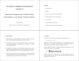
“A Course in Applied Econometrics” Lecture 15

Weak Instruments and Many Instruments

Guido Imbens IRP Lectures, UW Madison, August 2008 Outline

• 1. Introduction
• 2. Motivation
• 3. Weak Instruments
• 4. Many (Weak) Instruments

1

• 1. Introduction

Standard normal asymptotic approximation to sampling distri- bution of IV, TSLS, and LIML estimators relies on non-zero correlation between instruments and endogenous regressors. If correlation is close to zero, these approximations are not accurate even in fairly large samples. In the just identified case TSLS/LIML confidence intervals will still be fairly wide in most cases, even if not valid, unless degree

• f endogeneity is very high. If concerned with this, alternative

confidence intervals are available that are valid uniformly. No better estimators available.

2

In the case with large degree of overidentification TSLS has poor properties: considerable bias towards OLS, and substan- tial underestimation of standard errors. LIML is much better in terms of bias, but its standard error is not correct. A simple multiplicative adjustment to conventional LIML standard errors based on Bekker asymptotics or random effects likelihood works well. Overall: use LIML, with Bekker-adjusted standard errors.

3

SLIDE 2

2.A Motivation : Angrist-Krueger AK were interested in estimating the returns to years of edu-

• cation. Their basic specification is:

Yi = α + β · Ei + εi, where Yi is log (yearly) earnings and Ei is years of education. In an attempt to address the endogeneity problem AK exploit variation in schooling levels that arise from differential impacts

• f compulsory schooling laws by quarter of birth and use quarter
• f birth as an instrument. This leads to IV estimate (using only

1st and 4th quarter data): ˆ β = Y 4 − Y 1 E4 − E1 = 0.089 (0.011)

4

2.B AK with Many Instruments AK also present estimates based on additional instruments. They take the basic 3 qob dummies and interact them with 50 state and 9 year of birth dummies. Here (following Chamberlain and Imbens) we interact the single binary instrument with state times year of birth dummies to get 500 instruments. Also including the state times year of birth dummies as exogenous covariates leads to the following model: Yi = X′

iβ + εi,

E[Zi · εi] = 0, where Xi is the 501-dimensional vector with the 500 state/year dummies and years of education, and Zi is the vector with 500 state/year dummies and the 500 state/year dummies multiply- ing the indicator for the fourth quarter of birth.

5

The TSLS estimator for β is ˆ βTSLS = 0.073 (0.008) suggesting the extra instruments improve the standard errors a little bit. However, LIML estimator tells a somewhat different story, ˆ βLIML = 0.095 (0.017) with an increase in the standard error.

6

1.C Bound-Jaeger-Baker Critique BJB suggest that despite the large (census) samples used by AK asymptotic normal approximations may be very poor be- cause the instruments are only very weakly correlated with the endogenous regressor. The most striking evidence for this is based on the following

• calculation. Take the AK data and re-calculate their estimates

after replacing the actual quarter of birth dummies by random indicators with the same marginal distribution. In principle this means that the standard (gaussian) large sam- ple approximations for TSLS and LIML are invalid since they rely on non-zero correlations between the instruments and the endogenous regressor.

7

SLIDE 3

Single Instr 500 Instruments TSLS LIML Real QOB 0.089 (0.011) 0.073 (0.008) 0.095 (0.017) Random QOB

• 1.96

(18.12) 0.059 (0.009)

• 0.330

(0.100) With many random instruments the results are troubling. Al- though the instrument contains no information, the results sug- gest that the instruments can be used to infer precisely what the returns to education are.

8

1.D Simulations with a Single Instrument 10,000 artificial data sets, all of size 160,000, designed to mimic the AK data. In each of these data sets half the units have quarter of birth (denoted by Qi) equal to 0 and 1 respec- tively.

• νi

ηi

• ∼ N
• ,
• 0.446

ρ · √ 0.446 · √ 10.071 ρ · √ 0.446 · √ 10.071 10.071

• .

The correlation between the reduced form residuals in the AK data is ρ = 0.318. Ei = 12.688 + 0.151 · Qi + ηi, Yi = 5.892 + 0.014 · Qi + νi.

9

Now we calculate the IV estimator and its standard error, using either the actual qob variable or a random qob variable as the instrument. We are interested in the size of tests of the null that coefficient

• n years of education is equal to 0.089 = 0.014/0.151.

We base the test on the t-statistic. Thus we reject the null if the ratio of the point estimate minus 0.089 and the standard error is greater than 1.96 in absolute value. We repeat this for 12 different values of the reduced form error correlation. In Table 3 we report the coverage rate and the median and 0.10 quantile of the width of the estimated 95% confidence intervals.

10

Table 3: Coverage Rates of Conv. TSLS CI by Degree of Endogeneity

ρ 0.0 0.4 0.6 0.8 0.9 0.95 0.99 implied OLS 0.00 0.08 0.13 0.17 0.19 0.20 0.21 Real QOB Cov rate 0.95 0.95 0.96 0.95 0.95 0.95 0.95 Med Width 95% CI 0.09 0.08 0.07 0.06 0.05 0.05 0.05 0.10 quant Width 0.08 0.07 0.06 0.05 0.04 0.04 0.04 Random QOB Cov rate 0.99 1.00 1.00 0.98 0.92 0.82 0.53 Med Width 95% CI 1.82 1.66 1.45 1.09 0.79 0.57 0.26 0.10 quant Width 0.55 0.51 0.42 0.33 0.24 0.17 0.08

SLIDE 4

In this example, unless the reduced form correlations are very high, e.g., at least 0.95, with irrelevant instruments the conven- tional confidence intervals are wide and have good coverage. The amount of endogeneity that would be required for the conventional confidence intervals to be misleading is higher than one typically encounters in cross-section settings. Put differently, although formally conventional confidence in- tervals are not valid uniformly over the parameter space (e.g., Dufour, 1997), the subsets of the parameter space where re- sults are substantively misleading may be of limited interest. This in contrast to the case with many weak instruments where especially TSLS can be misleading in empirically relevant set- tings. 3.A Single Weak Instrument Yi = β0 + β1 · Xi + εi, Xi = π0 + π1 · Zi + ηi, with (εi, ηi) ⊥ ⊥ Zi, and jointly normal with covariance matrix Σ. The reduced form for the first equation is Yi = α0 + α1 · Zi + νi, where the parameter of interest is β1 = α1/π1. Let Ω = E

⎡ ⎣

• νi

ηi

• ·
• νi

ηi

′⎤ ⎦ ,

and Σ = E

⎡ ⎣

• εi

ηi

• ·
• εi

ηi

′⎤ ⎦ ,

13

Standard IV estimator: ˆ βIV

1

=

1 N N i=1

• Yi − Y

Zi − Z

• 1

N N i=1

• Xi − X

Zi − Z

,

Concentration parameter: λ = π2

1 · N

• i=1
• Zi − Z

2 /σ2 η.

14

Normal approximations for numerator and denominator are ac- curate: √ N

⎛ ⎝ 1

N

N

• i=1
• Yi − Y

Zi − Z

• − Cov(Yi, Zi)

⎞ ⎠ ≈ N (0, V (Yi · Zi)) ,

√ N

⎛ ⎝ 1

N

N

• i=1
• Xi − X

Zi − Z

• − Cov(Xi, ZI)

⎞ ⎠ ≈ N (0, V (Xi · Zi)) .

If π1 = 0, as the sample size gets large, then the ratio will eventually be well approximated by a normal distribution as well. However, if Cov(Xi, Zi) ≈ 0, the ratio may be better approx- imated by a Cauchy distribution, as the ratio of two normals centered close to zero.

15

SLIDE 5

3.B Staiger-Stock Asymptotics and Uniformity Staiger and Stock investigate the distribution of the standard IV estimator under an alternative asymptotic approximation. The standard asymptotics (strong instrument asymptotics in the SS terminology) is based on fixed parameters and the sam- ple size getting large. In their alternative asymptotic sequence SS model π1 as a func- tion of the sample size, π1N = c/ √ N, so that the concentration parameter converges to a constant: λ − → c2 · V (Zi). SS then compare coverage properties of various confidence in- tervals under this (weak instrument) asymptotic sequence.

16

The importance of the SS approach is in demonstrating for any sample size there are values of the nuisance parameters such that the actual coverage is substantially away from the nominal coverage. More recently the issue has therefore been reformulated as re- quiring confidence intervals to have asymptotically the correct coverage probabilities uniformly in the parameter space. See for a discussion from this perspective Mikusheva. Note that there cannot exist estimators that are consistent for β∗ uniformly in the parameter space since if π1 = 0, there are no consistent estimators for β1. However, for testing there are generally confidence intervals that are uniformly valid, but they are not of the conventional form, that is, a point estimate plus

• r minus a constant times a standard error.

17

3.C Anderson-Rubin Confidence Intervals Let the instrument ˜ Zi = Zi − Z be measured in deviations from its mean. Then define the statistic S(β1) = 1 N

N

• i=1

˜ Zi · (Yi − β1 · Xi) . Then, under the null hypothesis that β1 = β∗

1, and conditional

• n the instruments, the statistic

√ N ·S(β∗

1) has an exact normal

distribution √ N · S(β∗

1) ∼ N ⎛ ⎝0, N

• i=1

˜ Z2

i · σ2 ε ⎞ ⎠ .

18

Anderson and Rubin (1949) propose basing tests for the null hypothesis H0 : β1 = β0

1,

against the alternative hypothesis Ha : β1 = β0

1

• n this idea, through the statistic

AR

• β0

1

• = N · S(β0

1)2 N i=1 ˜

Z2

i

·

• 1

−β0

1

• Ω
• 1

−β0

1 −1

. A confidence interval can be based on this test statistic by inverting it: CIβ1

0.95 = {β1 |AR(β1) ≤ 3.84}

This interval can be equal to the whole real line.

19

SLIDE 6

3.D Anderson-Rubin with K instruments The reduced form is Xi = π0 + π′

1Zi + ηi,

S

• β0

1

• is now normally distributed vector.

AR statistic with associated confidence interval: AR

• β0

1

• = N · S
• β0

1 ′ ⎛ ⎝ N

• i=1

˜ Zi · ˜ Z′

i ⎞ ⎠ −1

S

• β0

1

• ·
• 1

−β0

1

• Ω
• 1

−β0

1

• CIβ1

0.95 =

• β1
• AR(β1) ≤ X2

0.95(K)

• ,

The problem is that this confidence interval can be empty be- cause it simultaneously tests validity of instruments.

20

3.E Kleibergen Test Kleibergen modfies AR statistic through ˜ S

• β0

1

• = 1

N

N

• i=1
• ˜

Z′

iˆ

π1(β0

1)

• ·
• Yi − β0

1 · Xi

• ,

where ˆ π is the maximum likelihood estimator for π1 under the restriction β1 = β0

• 1. The test is then based on the statistic

K

• β0

1

• = N · ˜

S(β0

1)2 N i=1 ˜

Z2

i

·

• 1

−β0

1

• Ω
• 1

−β0

1 −1

. This has an approximate chi-squared distribution, and can be used to construct a confidence interval.

21

3.F Moreira’s Similar Tests Moreira (2003) proposes a method for adjusting the critical values that applies to a number of tests, including the Kleiber- gen test. His idea is to focus on similar tests, test that have the same rejection probability for all values of the nuisance pa- rameter (the π) by adjusting critical values (instead of using quantiles from the chi-squared distribution). The way to adjust the critical values is to consider the distribu- tion of a statistic such as the Kleibergen statistic conditional

• n a complete sufficient statistic for the nuisance parameter.

In this setting a complete sufficient statistic is readily available in the form of the maximum likelihood estimator under the null, ˆ π1(β0

1).

22

Moreira’s preferred test is based on the likelihood ratio. Let LR

• β0

1

• = 2 ·
• L
• ˆ

β1, ˆ π

• − L
• β0

1, ˆ

π(β0

1)

• ,

be the likelihood ratio. Then let cLR(p, 0.95), be the 0.95 quantile of the distribution

• f LR(β0

1) under the null hypothesis, conditional on ˆ

π(β0

1) = p.

The proposed test is to reject the null hypothesis at the 5% level if LR

• β0

1

• > cLR(ˆ

π(β0

1), 0.95),

where conventional test would use critical values from a chi- squared distribution with a single degree of freedom. The crit- ical values are tabulated for low values of K. This test can then be converted to construct a 95% confidence intervals.

23

SLIDE 7

3.G Conditioning on the First Stage These confidence intervals are asymptotically valid irrespective

• f the strength of the first stage (the value of π1). However,

they are not valid if one first inspects the first stage, and con- ditional on the strength of that, decides to proceed. Specifically, if in practice one first inspects the first stage, and decide to abandon the project if the first stage F-statistic is less than some fixed value, and otherwise proceed by calculat- ing confidence interval, the large sample coverage probabilities would not be the nominal ones. Chioda and Jansson propose a confidence interval that is valid conditional on the strength of the first stage. A caveat is that this involves loss of information, and thus the Chioda-Jansson confidence intervals are wider than confidence intervals that are not valid conditional on the first stage.

24

4.A Many (Weak) Instruments In this section we discuss the case with many weak instruments. The problem is both the bias in the standard estimators, and the misleadingly small standard errors based on conventional procedures, leading to poor coverage rates for standard confi- dence intervals in many situations. Resampling methods such as bootstrapping do not solve these problems. The literature has taken a number of approaches. Part of the literature has focused on alternative confidence intervals analogues to the single instrument case. In addition a variety

• f new point estimators have been proposed.

Generally LIML still does well, but standard errors need to be adjusted.

25

4.B Bekker Asymptotics Bekker (1995) derives large sample approximations for TSLS and LIML based on sequences where the number of instruments increases proportionally to the sample size. He shows that TSLS is not consistent in that case. LIML is consistent, but the conventional LIML standard er- rors are not valid. Bekker then provides LIML standard errors that are valid under this asymptotic sequence. Even with rel- atively small numbers of instruments the differences between the Bekker and conventional asymptotics can be substantial.

26

Bekker correction, single endogenous regressor: Yi = β′

1X1i + β′ 2X2i + εi = β′Xi + εi,

X1i = π′

1Z1i + π′ 2X2i + ηi = π′Zi + ηi.

Define the matrices PZ and MZ as: PZ = Z(Z′Z)−1Z′, MZ = I − Z(Z′Z)−1Z′. Let σ2 be the variance of εi, with consistent estimator ˆ σ2. The standard TSLS variance is Vtsls = ˆ σ2 · (XPZX)−1 .

27

SLIDE 8

Under the standard, fixed number of instrument asymptotics, the asymptotic variance for LIML is identical to that for TSLS, and so in principle we can use the same estimator. In practice researchers typically estimate the variance for LIML as Vliml = ˆ σ2 ·

• XPZX − ˆ

λ · X′MZX

−1 .

28

To get Bekker’s correction, we need a little more notation. Define Ω =

• Y

X

• PZ
• Y

X

• /N =
• Ω11

Ω12 Ω′

12

Ω22

• ,

Ω11 = YPZY/N, Ω12 = YPZX/N, and Ω22 = XPZX/N. A = N · Ω′

12Ω12 − Ω22βΩ12 − Ω′ 12β′Ω22 + Ω22ββ′Ω22

Ω11 − 2Ω12β + β′Ω22β . Then: Vbekker = ˆ σ2 ·

• XPZX − ˆ

λ · X′MZX

−1

× (XPZX − λ · A) ·

• XPZX − ˆ

λ · X′MZX

−1 .

Recommended in practice

29

4.C Random Effects Estimators Chamberlain and Imbens propose a random effects quasi maxi- mum likelihood (REQML) estimator. They propose modelling the first stage coefficients πk, for k = 1, . . . , K, in the regression Xi = π0 + π′

1Zi + ηi = π0 + K

• k=1

πk · Zik + ηi, (after normalizing the instruments to have mean zero and unit variance,) as independent draws from a normal N(µπ, σ2

π) dis-

tribution.

30

Assuming also joint normality for (εi, ηi), one can derive the likelihood function L(β0, β1, π0, µπ, σ2

π, Ω).

In contrast to the likelihood function in terms of the original parameters (β0, β1, π0, π1, Ω), this likelihood function depends

• n a small set of parameters, and a quadratic approximation

to its logarithms is more likely to be accurate.

31

SLIDE 9

CI discuss some connections between the REQML estimator and LIML and TSLS in the context of this parametric set up. First they show that in large samples, with a large number of instruments, the TSLS estimator corresponds to the restricted maximum likelihood estimator where the variance of the first stage coefficients is fixed at a large number, or σ2

π = ∞:

ˆ βTSLS ≈ arg max

β0,β1,π0,µπ

= L(β0, β1, π0, µπ, σ2

π = ∞, Ω).

From a Bayesian perspective, TSLS corresponds approximately to the posterior mode given a flat prior on all the parameters, and thus puts a large amount of prior mass on values of the parameter space where the instruments are jointly powerful.

32

In the special case where we fix µπ = 0, and Ω is known, and the random effects specification applies to all instruments, CI show that the REQML estimator is identical to LIML. However, like the Bekker asymptotics, the REQML calculations suggests that the standard LIML variance is too small: the variance of the REQML estimator is approximately equal to the standard LIML variance times 1 + σ−2

π

·

⎛ ⎝

• 1

β1

′

Ω−1

• 1

β1

⎞ ⎠ −1

. This is similar to the Bekker adjustment.

33

4.D Choosing the Number of Instruments Donald and Newey (2001) consider the problem of choosing a subset of an infinite sequence of instruments. They assume the instruments are ordered, so that the choice is the number of instruments to use. The criterion they focus on is based on an estimable approx- imation to the expected squared error. version of this leads to approximately the same expected squared error as using the infeasible criterion. Although in its current form not straightforward to implement, this is a very promising approach that can apply to many related problems such as generalized method of moments settings with many moments.

34

4.E Flores’ Simulations In one of the more extensive simulation studies Flores-Lagunes reports results comparing TSLS, LIML, Fuller, Bias corrected versions of TSLS, LIML and Fuller, a Jacknife version of TSLS (Hahn, Hausman and Kuersteiner), and the REQML estimator, in settings with 100 and 500 observations, and 5 and 30 in- struments for the single endogenous variable. Does not include LIML with Bekker standard errors. He looks at median bias, median absolute error, inter decile range, coverage rates. He concludes that “our evidence indicates that the random- effects quasi-maximum likelihood estimator outperforms alter- native estimators in terms of median point estimates and cov- erage rates.”

35