A Course in Applied Econometrics 1. Introduction Lecture 10 2. - PowerPoint PPT Presentation
Outline A Course in Applied Econometrics 1. Introduction Lecture 10 2. Example I: Missing Data 3. Example II: Returns to Schooling Partial Identification 4. Example III: Initial Conditions Problems in Panel Data 5. Example IV: Auction
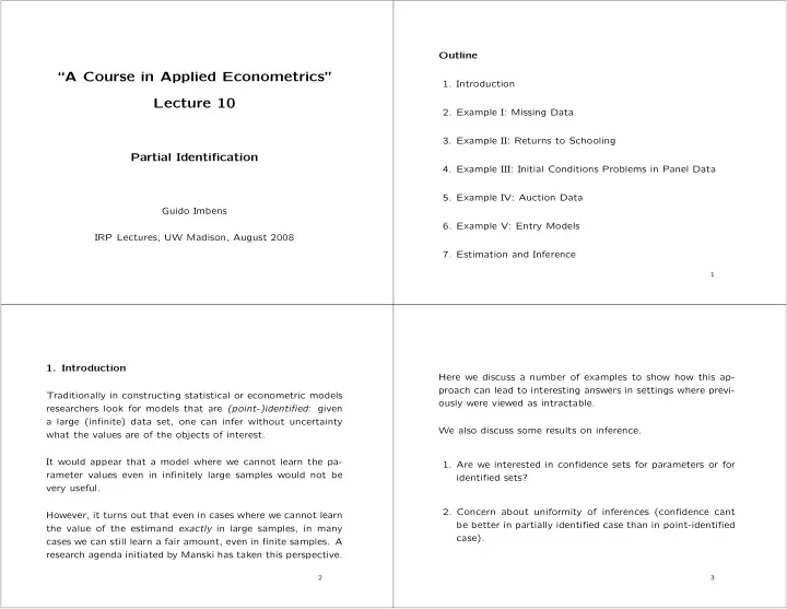
Outline “A Course in Applied Econometrics” 1. Introduction Lecture 10 2. Example I: Missing Data 3. Example II: Returns to Schooling Partial Identification 4. Example III: Initial Conditions Problems in Panel Data 5. Example IV: Auction Data Guido Imbens 6. Example V: Entry Models IRP Lectures, UW Madison, August 2008 7. Estimation and Inference 1 1. Introduction Here we discuss a number of examples to show how this ap- proach can lead to interesting answers in settings where previ- Traditionally in constructing statistical or econometric models ously were viewed as intractable. researchers look for models that are (point-)identified : given a large (infinite) data set, one can infer without uncertainty We also discuss some results on inference. what the values are of the objects of interest. It would appear that a model where we cannot learn the pa- 1. Are we interested in confidence sets for parameters or for rameter values even in infinitely large samples would not be identified sets? very useful. 2. Concern about uniformity of inferences (confidence cant However, it turns out that even in cases where we cannot learn be better in partially identified case than in point-identified the value of the estimand exactly in large samples, in many case). cases we can still learn a fair amount, even in finite samples. A research agenda initiated by Manski has taken this perspective. 2 3
2. I: Missing Data Now suppose we know that the variable of interest is binary: If D i = 1, we observe Y i , and if D i = 0 we do not observe Y i . Y i ∈ { 0 , 1 } . Then natural (not data-informed) lower and upper We always observe the missing data indicator D i . We assume the quantity of interest is the population mean θ = E [ Y i ]. bounds for µ 0 are 0 and 1 respectively. This implies bounds on θ : In large samples we can learn p = E [ D i ] and µ 1 = E [ Y i | D i = 1], but nothing about µ 0 = E [ Y i | D i = 0]. We can write: θ ∈ [ θ LB , θ UB ] = [ p · µ 1 , p · µ 1 + (1 − p )] . θ = p · µ 1 + (1 − p ) · µ 0 . These bounds are sharp , in the sense that without additional information we can not improve on them. Since even in large samples we learn nothing about µ 0 , it follows that without additional information there is no limit on the range of possible values for θ . Formally, for all values θ in [ θ LB , θ UB ], we can find a joint distri- bution of ( Y i , W i ) that is consistent with the joint distribution Even if p is very close to 1, the small probability that D i = 0 of the observed data and with θ . combined with the possibility that µ 0 is very large or very small allows for a wide range of values for θ . 4 5 We can also obtain informative bounds if we modify the object of interest a little bit. If fewer than 50% of the values are observed, or p < 1 / 2, Suppose we are interested in the median of Y i , θ 0 . 5 = med( Y i ). then we cannot learn anything about the median of Y i without additional information (for example, a bound on the values of Define q τ ( Y i ) to be the τ quantile of the conditional distribution Y i ), and the interval is ( −∞ , ∞ ). of Y i given D i = 1. Then the median cannot be larger than q 1 / (2 p ) ( Y i ) because even if all the missing values were large, we More generally, we can obtain bounds on the τ quantile of the know that at least p · (1 / (2 p )) = 1 / 2 of the units have a value distribution of Y i , equal to less than or equal to q 1 / (2 p ) ( Y i ). � � θ τ ∈ [ θ LB , θ UB ] = q ( τ − (1 − p )) /p ( Y i | D i = 1) , q τ/p ( Y i | D i = 1) . Then, if p > 1 / 2, we can infer that the median must satisfy which is bounded if the probability of Y i being missing is less � � θ 0 . 5 ∈ [ θ LB , θ UB ] = q (2 p − 1) / (2 p ) ( Y i ) , q 1 / (2 p ) ( Y i ) , than min( τ, 1 − τ ). and we end up with a well defined, and, depending on the data, more or less informative identified interval for the median. 6 7
3. Example II: Returns to Schooling Manski-Pepper are interested in estimating returns to school- Alternative Assumptions considered by MP ing. They start with an individual level response function Y i ( w ). Increasing education does not lower earnings: ∆( s, t ) = E [ Y i ( t ) − Y i ( s )] , is the difference in average outcomes (log earnings) given t Assumption 1 (Monotone Treatment Response) If w ′ ≥ w , then Y i ( w ′ ) ≥ Y i ( w ) . rather than s years of schooling. Values of ∆( s, t ) are the object of interest. On average, individuals who choose higher levels of education W i is the actual years of school, and Y i = Y i ( W i ) be the actual would have higher earnings at each level of education than log earnings. individuals who choose lower levels of education. If one makes an unconfoundedness/exogeneity assumption that Assumption 2 (Monotone Treatment Selection) Y i ( w ) ⊥ ⊥ W i | X i , If w ′′ ≥ w ′ , then for all w , E [ Y i ( w ) | W i = w ′′ ] ≥ E [ Y i ( w ) | W i = w ′ ] . for some set of covariates, one can estimate ∆( s, t ) consistently given some support conditions. MP relax this assumption. 8 9 Under these two assumptions, bound on E [ Y i ( w )] and ∆( s, t ): 4. Example III: Initial Conditions Problems in Panel Data (Honor´ e and Tamer) � E [ Y i | W i = w ] · Pr( W i ≥ w ) + E [ Y i | W i = v ] · Pr( W i = v ) v<w Y it = 1 { X ′ it β + Y it − 1 · γ + α i + ǫ it ≥ 0 } , ≤ E [ Y i ( w )] ≤ with the ǫ it independent N (0 , 1) over time and individuals. Fo- cus on γ . � E [ Y i | W i = w ] · Pr( W i ≤ w ) + E [ Y i | W i = v ] · Pr( W i = v ) . v>w Suppose we also postulate a parametric model for the random Using NLS data MP estimate the upper bound on the the effects α i : returns to four years of college, ∆(12 , 16) to be 0.397. α | X i 1 , . . . , X iT ∼ G ( α | θ ) Translated into average yearly returns this gives us 0.099, which is in fact lower than some estimates that have been Then the model is almost complete. reported in the literature. All that is missing is: This analysis suggests that the upper bound is in this case reasonably informative, given a remarkably weaker set of as- p ( Y i 1 | α i , X i 1 , . . . , X iT ) . sumptions. 10 11
HT assume a discrete distribution for α , with a finite and known set of support points. They fix the support to be − 3 , − 2 . 8 , . . . , 2 . 8 , 3, with unknown probabilities. In the case with T = 3 they find that the range of values for γ consistent with the data generating process (the identified set) is very narrow. If γ is in fact equal to zero, the width of the set is zero. If the true value is γ = 1, then the width of the interval is approximately 0.1. (It is largest for γ close to, but not equal to, -1.) See Figure 1, taken from HT. The HT analysis shows nicely the power of the partial identifi- cation approach: A problem that had been viewed as essentially intractable, with many non-identification results, was shown to admit potentially precise inferences. Point identification is not a big issue here. 12 5. Example IV: Auction Data Haile and Tamer study English or oral ascending bid auctions. In such auctions bidders offer increasingly higher prices until only one bidder remains. HT focus on a symmetric independent Haile-Tamer Assumptions private values model. In auction t , bidder i has a value ν it , drawn independently from the value for bidder j , with cdf F ν ( v ) Assumption 3 No bidder ever bids more than their valuation HT are interested in the value distribution F ν ( v ). This is as- sumed to be the same in each auction (after adjusting for Assumption 4 No bidder will walk away and let another bidder observable auction characteristics). win the auction if the winning bid is lower than their own valuation One can imagine observing exactly when each bidder leaves the auction, thus directly observing their valuations. This is not what is typically observed. For each bidder we do not know at any point in time whether they are still participating unless they subsequently make a higher bid. 13 14
Recommend
More recommend
Explore More Topics
Stay informed with curated content and fresh updates.
