CS70: Jean Walrand: Lecture 29. Confidence? Confidence? Confidence - PowerPoint PPT Presentation

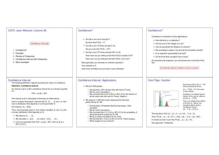
CS70: Jean Walrand: Lecture 29. Confidence? Confidence? Confidence is essential is many applications: ◮ You flip a coin once and get H . ◮ How effective is a medication? Do think that Pr [ H ] = 1? Confidence Intervals ◮ Are we sure of the milage of a car? ◮ You flip a coin 10 times and get 5 H s. ◮ Can we guarantee the lifespan of a device? Are you sure that Pr [ H ] = 0 . 5? ◮ We simulated a system. Do we trust the simulation results? 1. Confidence? ◮ You flip a coin 10 6 times and get 35 % of H s. 2. Example ◮ Is an algorithm guaranteed to be fast? How much are you willing to bet that Pr [ H ] is exactly 0 . 35? 3. Review of Chebyshev ◮ Do we know that a program has no bug? How much are you willing to bet that Pr [ H ] ∈ [ 0 . 3 , 0 . 4 ] ? 4. Confidence Interval with Chebyshev As scientists and engineers, you should become convinced of this 5. More examples More generally, you estimate an unknown quantity θ . fact: Your estimate is ˆ θ . An estimate without confidence level is useless! How much confidence do you have in your estimate? Confidence Interval Confidence Interval: Applications Coin Flips: Intuition The following definition captures precisely the notion of confidence. Say that you flip a coin n = 100 Definition: Confidence Interval ◮ We poll 1000 people. times and observe 20 Hs. An interval [ a , b ] is a 95 % -confidence interval for an unknown quantity ◮ Among those, 48 % declare they will vote for Trump. If p := Pr [ H ] = 0 . 5, this event θ if is very unlikely. ◮ We do some calculations .... Pr [ θ ∈ [ a , b ]] ≥ 95 % . ◮ We conclude that [ 0 . 43 , 0 . 53 ] is a 95 % -CI for the fraction of Intuitively, if is unlikely that the all the voters who will vote for Trump. (Arghhh.) fraction of Hs, say A n , differs a lot from p := Pr [ H ] . The interval [ a , b ] is calculated on the basis of observations. ◮ We observe 1 , 000 heart valve replacements that were Thus, it is unlikely that p differs Here is a typical framework. Assume that X 1 , X 2 ,..., X n are i.i.d. and performed by Dr. Bill. a lot from A n . Hence, one have a distribution that depends on some parameter θ . should be able to build a ◮ Among those, 35 patients died during surgery. (Sad For instance, X n = B ( θ ) . confidence interval example!) [ A n − δ , A n + δ ] for p . ◮ We do some calculations ... Thus, more precisely, given θ , the random variables X n are i.i.d. with a known distribution (that depends on θ ). ◮ We conclude that [ 1 % , 5 %] is a 95 % -CI for the probability of The key idea is that | A n − p | ≤ δ ⇔ p ∈ [ A n − δ , A n + δ ] . dying during that surgery by Dr. Bill. ◮ We observe X 1 ,..., X n ◮ We do a similar calculation for Dr. Fred. Thus, Pr [ | A n − p | > δ ] ≤ 5 % ⇔ Pr [ p ∈ [ A n − δ , A n + δ ]] ≥ 95 % . ◮ We calculate a = a ( X 1 ,..., X n ) and b = b ( X 1 ,..., X n ) ◮ We find that [ 8 % , 12 %] is a 95 % -CI for Dr. Fred’s surgery. It remains to find δ such that Pr [ | A n − p | > δ ] ≤ 5 % . ◮ What surgeon do you choose? ◮ If we can guarantee that Pr [ θ ∈ [ a , b ]] ≥ 95 % , then [ a , b ] is a One approach: Chebyshev. 95 % -CI for θ .

Confidence Interval with Chebyshev Confidence Intervals: Result Confidence Interval: Analysis We prove the theorem, i.e., that A n ± 4 . 5 σ / √ n is a 95 % -CI for µ . From Chebyshev: Theorem: √ Let X n be i.i.d. with mean µ and variance σ 2 . var ( A n ) n Pr [ | A n − µ | ≥ 4 . 5 σ / n ] ≤ [ 4 . 5 σ / √ n ] 2 = 20 σ 2 var ( A n ) . ◮ Flip a coin n times. Let A n be the fraction of H s. Define A n = X 1 + ··· + X n . Then, n ◮ Can we find δ such that Pr [ | A n − p | > δ ] ≤ 5 % ? Now, Pr [ µ ∈ [ A n − 4 . 5 σ √ n , A n + 4 . 5 σ √ n ]] ≥ 95 % . var ( X 1 + ··· + X n ) = 1 Using Chebyshev, we will see that δ = 2 . 25 1 var ( A n ) = n 2 var ( X 1 + ··· + X n ) √ n works. Thus n Thus, [ A n − 4 . 5 σ √ n , A n + 4 . 5 σ √ n ]] is a 95 % -CI for µ . n 2 × n . var ( X 1 ) = 1 1 n σ 2 . [ A n − 2 . 25 √ n , A n + 2 . 25 = √ n ] is a 95%-CI for p . Hence, Example: Let X n = 1 { coin n yields H } . Then √ 20 σ 2 × 1 n n σ 2 = 5 % . Pr [ | A n − µ | ≥ 4 . 5 σ / n ] ≤ Example: If n = 1500, then Pr [ p ∈ [ A n − 0 . 05 , A n + 0 . 05 ]] ≥ 95 % . µ = E [ X n ] = p := Pr [ H ] . Also, σ 2 = var ( X n ) = p ( 1 − p ) ≤ 1 4 . 1 In fact, we will see later that a = √ n works, so that with n = 1 , 500 one has Thus, √ Pr [ p ∈ [ A n − 0 . 02 , A n + 0 . 02 ]] ≥ 95 % . Pr [ | A n − µ | ≤ 4 . 5 σ / n ] ≥ 95 % . Hence, [ A n − 4 . 5 1 / 2 √ n , A n + 4 . 5 1 / 2 √ n ]] is a 95 % -CI for p . Hence, √ √ Pr [ µ ∈ [ A n − 4 . 5 σ / n , A n + 4 . 5 σ / n ]] ≥ 95 % . Confidence interval for p in B ( p ) Confidence interval for p in B ( p ) Confidence interval for p in B ( p ) Let X n be i.i.d. B ( p ) . Define A n = ( X 1 + ··· + X n ) / n . Theorem: An illustration: Improved CI: Later we will see that we can replace 2 . 25 by 1. [ A n − 2 . 25 √ n , A n + 2 . 25 √ n ] is a 95%-CI for p . Proof: We have just seen that √ √ Pr [ µ ∈ [ A n − 4 . 5 σ / n , A n + 4 . 5 σ / n ]] ≥ 95 % . Here, µ = p and σ 2 = p ( 1 − p ) . Thus, σ 2 ≤ 1 4 and σ ≤ 1 2 . Thus, Good practice: You run your simulation, or experiment. You get an Quite a bit of work to get there: continuous random variables; √ √ estimate. You indicate your confidence interval. Gaussian; Central Limit Theorem. Pr [ µ ∈ [ A n − 4 . 5 × 0 . 5 / n , A n + 4 . 5 × 0 . 5 / n ]] ≥ 95 % .

Confidence Interval for 1 / p in G ( p ) Which Coin is Better? Unknown σ � You are given coin A and coin B . You want to find out which one has For B ( p ) , we wanted to estimate p . The CI requires σ = p ( 1 − p ) . We Let X n be i.i.d. G ( p ) . Define A n = ( X 1 + ··· + X n ) / n . replaced σ by an upper bound: 1 / 2. a larger Pr [ H ] . Let p A and p B be the values of Pr [ H ] for the two coins. Theorem: In some applications, it may be OK to replace σ 2 by the following sample Approach: A n 1 − 4 . 5 / √ n ] is a 95%-CI for 1 A n variance: [ 1 + 4 . 5 / √ n , p . ◮ Flip each coin n times. n n := 1 ◮ Let A n be the fraction of Hs for coin A and B n for coin B . s 2 ( X m − A n ) 2 . ∑ n m = 1 Proof: We know that ◮ Assume A n > B n . It is tempting to think that p A > p B . However, in some cases, this is dangerous! The theory says it is OK if the Confidence? √ √ Pr [ µ ∈ [ A n − 4 . 5 σ / n , A n + 4 . 5 σ / n ]] ≥ 95 % . distribution of X n is nice (Gaussian). This is used regularly in practice. Analysis: Note that However, be aware of the risk. √ 1 − p E [ A n − B n ] = p A − p B and var ( A n − B n ) = 1 n ( p A ( 1 − p A )+ p B ( 1 − p B )) ≤ 1 Here, µ = 1 ≤ 1 p and σ = p . Hence, 2 n . p Pr [ 1 1 1 p √ n , A n + 4 . 5 p √ n ]] ≥ 95 % . p ∈ [ A n − 4 . 5 1 Thus, Pr [ | A n − B n − ( p A − p B ) | > δ ] ≤ 2 n δ 2 , so p √ n ≤ 1 1 p ≤ 1 1 Now, A n − 4 . 5 p ≤ A n + 4 . 5 p √ n is equivalent to 1 Pr [ p A − p B ∈ [ A n − B n − δ , A n − B n + δ ]] ≥ 1 − 2 n δ 2 , and 1 + 4 . 5 / √ n ≤ 1 A n A n p ≤ 1 − 4 . 5 / √ n . 1 Pr [ p A − p B ≥ 0 ] ≥ 1 − 2 n ( A n − B n ) 2 . Examples: [ 0 . 7 A 100 , 1 . 8 A 100 ] and [ 0 . 96 A 10000 , 1 . 05 A 10000 ] . Example: With n = 100 and A n − B n = 0 . 2, Pr [ p A > p B ] ≥ 1 − 1 8 = 0 . 875 . Summary Confidence Intervals 1. Estimates without confidence level are useless! 2. [ a , b ] is a 95 % -CI for θ if Pr [ θ ∈ [ a , b ]] ≥ 95 % . 3. Using Chebyshev: [ A n − 4 . 5 σ / √ n , A n + 4 . 5 σ / √ n ] is a 95 % -CI for µ . 4. Using CLT, we will replace 4 . 5 by 2. 5. When σ is not known, one can replace it by an upper bound. 6. Examples: B ( p ) , G ( p ) , which coin is better? 7. In some cases, one can replace σ by the empirical standard deviation.