CS70: Jean Walrand: Lecture 25. Balls and Coupons & Random - PowerPoint PPT Presentation
CS70: Jean Walrand: Lecture 25. Balls and Coupons & Random Variables Coupons Random Variables Balls and Coupons: Key Results 1) Balls: Throw m balls into n > m bins. Pr [ no collision ] exp { m 2 2 n } . E.g., Pr [ 60 people
CS70: Jean Walrand: Lecture 25. Balls and Coupons & Random Variables ◮ Coupons ◮ Random Variables
Balls and Coupons: Key Results 1) Balls: Throw m balls into n > m bins. Pr [ no collision ] ≈ exp {− m 2 2 n } . E.g., Pr [ 60 people have different birthdays ] ≈ exp {− ( 60 ) 2 2 × 365 } ≈ 0 . 007. 2) Coupons: n ≫ 1 different baseball card; one at random in a cereal box. You buy m boxes. Pr [ miss a specific card ] ≈ exp {− m n } ; Pr [ miss at least one card ] ≤ n exp {− m n } . E.g., if n = 1000 and m = 7600 , then Pr [ miss at least one card ] ≤ 0 . 5.
Balls: Derivation 1) Balls: Throw m balls into n > m bins. Pr [ no collision ] ≈ exp {− m 2 2 n } . Preliminary Fact: ln ( 1 − ε ) ≈ − ε for | ε | ≪ 1. Define B k := ‘no collision in first k balls’ = ‘first k balls in k different bins’ . Then, α := Pr [ no collision in m balls ] = Pr [ B 1 ∩ B 2 ∩···∩ B m ] = Pr [ B 1 ] Pr [ B 2 | B 1 ] ··· P [ B m | B 1 ∩ B 2 ∪···∩ B m − 1 ] = 1 × ( 1 − 1 n ) × ( 1 − 2 n ) ×···× ( 1 − m − 1 ) . n Hence, ln ( 1 − 1 n )+ ··· + ln ( 1 − m − 1 ln ( α ) = ) n ≈ − m 2 − 1 n −···− m − 1 ≈ 2 n . n
Coupons: Derivations 2) Coupons: n ≫ 1 different baseball card; one at random in a cereal box. You buy m boxes. Pr [ miss a specific card ] ≈ exp {− m n } ; Pr [ miss at least one card ] ≤ n exp {− m n } . a) β := Pr [ miss a specific card ] = ( 1 − 1 n ) m . ln ( β ) = m ln ( 1 − 1 n ) ≈ − m n . Hence, β ≈ exp {− m n } . b) Let A := ‘miss at least one card’ and A k := ‘miss card k ’. n Pr [ A k ] ≈ n exp {− m A = ∪ n ∑ k = 1 A k ⇒ Pr [ A ] ≤ n } . k = 1
Random Variables: Questions about outcomes ... ◮ Experiment: roll two dice. Sample Space: { ( 1 , 1 ) , ( 1 , 2 ) ,..., ( 6 , 6 ) } = { 1 ,..., 6 } 2 How many pips? ◮ Experiment: flip 100 coins. Sample Space: { HHH ··· H , THH ··· H ,..., TTT ··· T } How many heads in 100 coin tosses? ◮ Experiment: choose a random student in cs70. Sample Space: { Adam , Jin , Bing ,..., Angeline } What midterm score? ◮ Experiment: hand back assignments to 3 students at random. Sample Space: { 123 , 132 , 213 , 231 , 312 , 321 } How many students get back their own assignment? ◮ In each scenario, each outcome gives a number. The number is a (known) function of the outcome.
Random Variables. A random variable, X , for an experiment with sample space Ω is a function X : Ω → ℜ . Thus, X ( · ) assigns a real number X ( ω ) to each ω ∈ Ω . The function X ( · ) is defined on the outcomes Ω . The function X ( · ) is not random, not a variable! What varies at random (from experiment to experiment)? The outcome!
Example 1 of Random Variable Experiment: roll two dice. Sample Space: { ( 1 , 1 ) , ( 1 , 2 ) ,..., ( 6 , 6 ) } = { 1 ,..., 6 } 2 Random Variable X : number of pips. X ( 1 , 1 ) = 2 X ( 1 , 2 ) = 3, . . . X ( 6 , 6 ) = 12, X ( a , b ) = a + b , ( a , b ) ∈ Ω .
Example 2 of Random Variable Experiment: flip three coins Sample Space: { HHH , THH , HTH , TTH , HHT , THT , HTT , TTT } Winnings: if win 1 on heads, lose 1 on tails: X X ( HHH ) = 3 X ( THH ) = 1 X ( HTH ) = 1 X ( TTH ) = − 1 X ( HHT ) = 1 X ( THT ) = − 1 X ( HTT ) = − 1 X ( TTT ) = − 3
Number of pips in two dice. “What is the likelihood of getting n pips?” Pr [ X = 10 ] = 3 / 36 = Pr [ X − 1 ( 10 )]; Pr [ X = 8 ] = 5 / 36 = Pr [ X − 1 ( 8 )] .
Distribution The probability of X taking on a value a . Definition: The distribution of a random variable X , is { ( a , Pr [ X = a ]) : a ∈ A } , where A is the range of X . Pr [ X = a ] := Pr [ X − 1 ( a )] where X − 1 ( a ) := { ω | X ( ω ) = a } .
Handing back assignments Experiment: hand back assignments to 3 students at random. Sample Space: Ω = { 123 , 132 , 213 , 231 , 312 , 321 } How many students get back their own assignment? Random Variable: values of X ( ω ) : { 3 , 1 , 1 , 0 , 0 , 1 } Distribution: 0 , w.p. 1 / 3 X = 1 , w.p. 1 / 2 0 . 4 3 , w.p. 1 / 6 0 . 2 0 0 1 2 3
Flip three coins Experiment: flip three coins Sample Space: { HHH , THH , HTH , TTH , HHT , THT , HTT , TTT } Winnings: if win 1 on heads, lose 1 on tails. X Random Variable: { 3 , 1 , 1 , − 1 , 1 , − 1 , − 1 , − 3 } Distribution: − 3 , w. p. 1 / 8 − 1 , w. p. 3 / 8 0 . 4 X = 1 , w. p. 3 / 8 0 . 3 3 w. p. 1 / 8 0 . 2 0 . 1 0 − 3 − 2 − 1 0 1 2 3
Number of pips. Experiment: roll two dice.
The binomial distribution. Flip n coins with heads probability p . Random variable: number of heads. Binomial Distribution: Pr [ X = i ] , for each i . How many sample points in event “ X = i ”? � n � i heads out of n coin flips = ⇒ i What is the probability of ω if ω has i heads? Probability of heads in any position is p . Probability of tails in any position is ( 1 − p ) . So, we get Pr [ ω ] = p i ( 1 − p ) n − i . Probability of “ X = i ” is sum of Pr [ ω ] , ω ∈ “ X = i ”. � n � p i ( 1 − p ) n − i , i = 0 , 1 ,..., n : B ( n , p ) distribution Pr [ X = i ] = i
The binomial distribution.
Binomial Distribution. Here are some examples:
Combining Random Variables. Let X and Y be two RV on the same probability space. That is, X : Ω → ℜ assigns the value X ( ω ) to ω . Also, Y : Ω → ℜ assigns the value Y ( ω ) to ω . Then X + Y is a random variable: It assigns the value X ( ω )+ Y ( ω ) to ω . Experiment: Roll two dice. X = outcome of first die, Y = outcome of second die. Thus, X ( a , b ) = a and Y ( a , b ) = b for ( a , b ) ∈ Ω = { 1 ,..., 6 } 2 . Then Z = X + Y = sum of two dice is defined by Z ( a , b ) = X ( a , b )+ Y ( a , b ) = a + b .
Combining Random Variables Other random variables: ◮ X k : Ω → ℜ is defined by X k ( ω ) = [ X ( ω )] k . In the dice example, X 3 ( a , b ) = a 3 . ◮ ( X − 2 ) 2 + 4 XY assigns the value ( X ( ω ) − 2 ) 2 + 4 X ( ω ) Y ( ω ) to ω . ◮ g ( X , Y , Z ) assigned the value g ( X ( ω ) , Y ( ω ) , Z ( ω )) to ω .
Expectation. How did people do on the midterm? Distribution. Summary of distribution? Average!
Expectation - Intuition Flip a loaded coin with Pr [ H ] = p a large number N of times. We expect heads to come up a fraction p of the times and tails a fraction 1 − p . Say that you get 5 for every H and 3 for every T . If there are N ( H ) outcomes equal to H and N ( T ) outcomes equal to T , you collect 5 × N ( H )+ 3 × N ( T ) . pause You average gain per experiment is then 5 N ( H )+ 3 N ( T ) . N Since N ( H ) ≈ p = Pr [ X = 5 ] and N ( T ) ≈ 1 − p = Pr [ X = 3 ] , we N N find that the average gain per outcome is approximately equal to 5 Pr [ X = 5 ]+ 3 Pr [ X = 3 ] . We use this frequentist interpretation as a definition.
Expectation - Definition Definition: The expected value of a random variable X is E [ X ] = ∑ a × Pr [ X = a ] . a The expected value is also called the mean. According to our intuition, we expect that if we repeat an experiment a large number N of times and if X 1 ,..., X N are the successive values of the random variable, then X 1 + ··· + X N ≈ E [ X ] . N That is indeed the case, in the same way that the fraction of times that X = x approaches Pr [ X = x ] . This (nontrivial) result is called the Law of Large Numbers. The subjectivist interpretation of E [ X ] is less obvious.
Expectation: A Useful Fact Theorem: E [ X ] = ∑ X ( ω ) × Pr [ ω ] . ω Proof: = ∑ E [ X ] a × Pr [ X = a ] a = ∑ ∑ a × Pr [ ω ] a ω : X ( ω )= a = ∑ ∑ X ( ω ) Pr [ ω ] a ω : X ( ω )= a = ∑ X ( ω ) Pr [ ω ] ω
An Example Flip a fair coin three times. Ω = { HHH , HHT , HTH , THH , HTT , THT , TTH , TTT } . X = number of H ’s: { 3 , 2 , 2 , 2 , 1 , 1 , 1 , 0 } . Thus, X ( ω ) Pr [ ω ] = { 3 + 2 + 2 + 2 + 1 + 1 + 1 + 0 }× 1 ∑ 8 . ω Also, a × Pr [ X = a ] = 3 × 1 8 + 2 × 3 8 + 1 × 3 8 + 0 × 1 ∑ 8 . a
Expectation and Average. There are n students in the class; X ( m ) = score of student m , for m = 1 , 2 ,..., n . “Average score” of the n students: add scores and divide by n : Average = X ( 1 )+ X ( 1 )+ ··· + X ( n ) . n Experiment: choose a student uniformly at random. Uniform sample space: Ω = { 1 , 2 , ··· , n } , Pr [ ω ] = 1 / n , for all ω . Random Variable: midterm score: X ( ω ) . Expectation: X ( ω ) 1 E ( X ) = ∑ X ( ω ) Pr [ ω ] = ∑ n . ω ω Hence, Average = E ( X ) . This holds for a uniform probability space.
Handing back assignments We give back assignments randomly to three students. What is the expected number of students that get their own assignment back? “The expected number of fixed points in a random permutation.” Expected value of a random variable: E [ X ] = ∑ a × Pr [ X = a ] . a For 3 students (permutations of 3 elements): Pr [ X = 3 ] = 1 / 6 , Pr [ X = 1 ] = 1 / 2 , Pr [ X = 0 ] = 1 / 3 . E [ X ] = 3 × 1 6 + 1 × 1 2 + 0 × 1 3 = 1 .
Win or Lose. Expected winnings for heads/tails games, with 3 flips? E [ X ] = 3 × 1 8 + 1 × 3 8 − 1 × 3 8 − 3 × 1 8 = 0 . Can you ever win 0? Apparently: expected value is not a common value, by any means.
Recommend
More recommend
Explore More Topics
Stay informed with curated content and fresh updates.
