CS70: Jean Walrand: Lecture 35. Conditional Expectation, Continuous - PowerPoint PPT Presentation

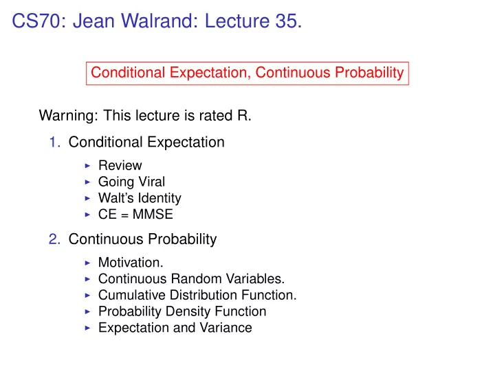
CS70: Jean Walrand: Lecture 35. Conditional Expectation, Continuous Probability Warning: This lecture is rated R. 1. Conditional Expectation ◮ Review ◮ Going Viral ◮ Walt’s Identity ◮ CE = MMSE 2. Continuous Probability ◮ Motivation. ◮ Continuous Random Variables. ◮ Cumulative Distribution Function. ◮ Probability Density Function ◮ Expectation and Variance

Conditional Expectation Definition Let X and Y be RVs on Ω . The conditional expectation of Y given X is defined as E [ Y | X ] = g ( X ) where g ( x ) := E [ Y | X = x ] := ∑ yPr [ Y = y | X = x ] . y

Properties of Conditional Expectation E [ Y | X = x ] = ∑ yPr [ Y = y | X = x ] y Theorem (a) X , Y independent ⇒ E [ Y | X ] = E [ Y ] ; (b) E [ aY + bZ | X ] = aE [ Y | X ]+ bE [ Z | X ] ; (c) E [ Yh ( X ) | X ] = h ( X ) E [ Y | X ] , ∀ h ( · ) ; (d) E [ h ( X ) E [ Y | X ]] = E [ h ( X ) Y ] , ∀ h ( · ) ; (e) E [ E [ Y | X ]] = E [ Y ] .

Application: Going Viral Consider a social network (e.g., Twitter). You start a rumor (e.g., Walrand is really weird). You have d friends. Each of your friend retweets w.p. p . Each of your friends has d friends, etc. Does the rumor spread? Does it die out (mercifully)? In this example, d = 4.

Application: Going Viral Fact: Let X = ∑ ∞ n = 1 X n . Then, E [ X ] < ∞ iff pd < 1 . Proof: Given X n = k , X n + 1 = B ( kd , p ) . Hence, E [ X n + 1 | X n = k ] = kpd . Thus, E [ X n + 1 | X n ] = pdX n . Consequently, E [ X n ] = ( pd ) n − 1 , n ≥ 1 . If pd < 1, then E [ X 1 + ··· + X n ] ≤ ( 1 − pd ) − 1 = ⇒ E [ X ] ≤ ( 1 − pd ) − 1 . If pd ≥ 1, then for all C one can find n s.t. E [ X ] ≥ E [ X 1 + ··· + X n ] ≥ C . In fact, one can show that pd ≥ 1 = ⇒ Pr [ X = ∞ ] > 0.

Application: Going Viral An easy extension: Assume that everyone has an independent number D i of friends with E [ D i ] = d . Then, the same fact holds. To see this, note that given X n = k , and given the numbers of friends D 1 = d 1 ,..., D k = d k of these X n people, one has X n + 1 = B ( d 1 + ··· + d k , p ) . Hence, E [ X n + 1 | X n = k , D 1 = d 1 ,..., D k = d k ] = p ( d 1 + ··· + d k ) . Thus, E [ X n + 1 | X n = k , D 1 ,..., D k ] = p ( D 1 + ··· + D k ) . Consequently, E [ X n + 1 | X n = k ] = E [ p ( D 1 + ··· + D k )] = pdk . Finally, E [ X n + 1 | X n ] = pdX n , and E [ X n + 1 ] = pdE [ X n ] . We conclude as before.

Application: Wald’s Identity Here is an extension of an identity we used in the last slide. Theorem Wald’s Identity Assume that X 1 , X 2 ,... and Z are independent, where Z takes values in { 0 , 1 , 2 ,... } and E [ X n ] = µ for all n ≥ 1. Then, E [ X 1 + ··· + X Z ] = µ E [ Z ] . Proof: E [ X 1 + ··· + X Z | Z = k ] = µ k . Thus, E [ X 1 + ··· + X Z | Z ] = µ Z . Hence, E [ X 1 + ··· + X Z ] = E [ µ Z ] = µ E [ Z ] .

CE = MMSE Theorem E [ Y | X ] is the ‘best’ guess about Y based on X . Specifically, it is the function g ( X ) of X that minimizes E [( Y − g ( X )) 2 ] .

CE = MMSE Theorem CE = MMSE g ( X ) := E [ Y | X ] is the function of X that minimizes E [( Y − g ( X )) 2 ] . Proof: First recall the projection property of CE: E [( Y − E [ Y | X ]) h ( X )] = 0 , ∀ h ( · ) . That is, the error Y − E [ Y | X ] is orthogonal to any h ( X ) .

CE = MMSE Theorem CE = MMSE g ( X ) := E [ Y | X ] is the function of X that minimizes E [( Y − g ( X )) 2 ] . Proof: Let h ( X ) be any function of X . Then E [( Y − h ( X )) 2 ] E [( Y − g ( X )+ g ( X ) − h ( X )) 2 ] = E [( Y − g ( X )) 2 ]+ E [( g ( X ) − h ( X )) 2 ] = + 2 E [( Y − g ( X ))( g ( X ) − h ( X ))] . But, E [( Y − g ( X ))( g ( X ) − h ( X ))] = 0 by the projection property . Thus, E [( Y − h ( X )) 2 ] ≥ E [( Y − g ( X )) 2 ] .

E [ Y | X ] and L [ Y | X ] as projections L [ Y | X ] is the projection of Y on { a + bX , a , b ∈ ℜ } : LLSE E [ Y | X ] is the projection of Y on { g ( X ) , g ( · ) : ℜ → ℜ } : MMSE.

Continuous Probability - James Bond. ◮ Escapes from SPECTRE sometime during 1 , 000 mile flight. ◮ Uniformly likely to be at any point along path. What is the chance he is at any point along the path? Discrete Setting: Uniorm over Ω = { 1 ,..., 1000 } . Continuous setting: probability at any point in [ 0 , 1000 ] ? Probability at any one of an infinite number of points is .. ...uh ...0?

Continuous Probability: the interval! Consider [ a , b ] ⊆ [ 0 ,ℓ ] (for James, ℓ = 1000 . ) Let [ a , b ] also denote the event that point is in the interval [ a , b ] . Pr [[ a , b ]] = length of [ a , b ] length of [ 0 ,ℓ ] = b − a = b − a 1000 . ℓ Again, [ a , b ] ⊆ Ω = [ 0 ,ℓ ] are events. Events in this space are unions of intervals. Example: the event A - “within 50 miles of base” is [ 0 , 50 ] ∪ [ 950 , 1000 ] . Pr [ A ] = Pr [[ 0 , 50 ]]+ Pr [[ 950 , 10000 ]] = 1 10 .

Shooting.. Another Bond example: Spectre is chasing him in a buggie. Bond shoots at buggy and hits it at random spot. What is the chance he hits gas tank? Gas tank is a one foot circle and the buggy is 4 × 5 rectangle. buggy gas Ω = { ( x , y ) : x ∈ [ 0 , 4 ] , y ∈ [ 0 , 5 ] } . The size of the event is π ( 1 ) 2 = π . The “size” of the sample space which is 4 × 5 . Since uniform, probability of event is π 20 .

Buffon’s needle. Throw a needle on a board with horizontal lines at random. Lines 1 unit apart, needle has length 1. What is the probability that the needle hits a line? Clearly... 2 π .

Buffon’s needle. Sample space: possible positions of needle. Position: center position ( X , Y ) , orientation, Θ . Θ · ( X , Y ) Y Relevant: X coordinate .. doesn’t matter; Y coordinate := distance from closest line. Y ∈ [ 0 , 1 2 ] ; Θ := closest angle to vertical [ − π 2 , π 2 ] . When Y ≤ 1 2 cos Θ : needle intersects line. � π / 2 � Pr [Θ ∈ [ θ , θ + d θ ]] Pr [ Y ≤ 1 � Pr [ “intersects” ] = 2 cos θ ] − π / 2 � π / 2 � [ d θ π ] × [( 1 / 2 ) cos θ � = 2 π [ 1 − π / 2 = 2 2 sin θ ] π / 2 = ] π . 1 / 2 − π / 2

Continuous Random Variables: CDF Pr [ a ≤ X ≤ b ] instead of Pr [ X = a ] . For all a and b specifies the behavior! Simpler: P [ X ≤ x ] for all x . Cumulative probability Distribution Function of X is F ( x ) = Pr [ X ≤ x ] Pr [ a < X ≤ b ] = Pr [ X ≤ b ] − Pr [ X ≤ a ] = F ( b ) − F ( a ) . Idea: two events X ≤ b and X ≤ a . Difference is the event a ≤ X ≤ b .

Example: CDF Example: Bond’s position.  0 for x < 0  x F ( x ) = Pr [ X ≤ x ] = for 0 ≤ x ≤ 1000 1000 1 for x > 1000  Probability that Bond is within 50 miles of center: Pr [ 450 < X ≤ 550 ] = Pr [ X ≤ 550 ] − Pr [ X ≤ 450 ] 1000 − 450 550 = 1000 1000 = 1 100 = 10

Example: CDF Example: hitting random location on gas tank. Random location on circle. 1 y Random Variable: Y distance from center. Probability within y of center: area of small circle Pr [ Y ≤ y ] = area of dartboard π y 2 = y 2 . = π Hence,  0 for y < 0  y 2 F Y ( y ) = Pr [ Y ≤ y ] = for 0 ≤ y ≤ 1 1 for y > 1 

Calculation of event with dartboard.. Probability between . 5 and . 6 of center? Recall CDF .  0 for y < 0  y 2 F Y ( y ) = Pr [ Y ≤ y ] = for 0 ≤ y ≤ 1 1 for y > 1  Pr [ 0 . 5 < Y ≤ 0 . 6 ] = Pr [ Y ≤ 0 . 6 ] − Pr [ Y ≤ 0 . 5 ] = F Y ( 0 . 6 ) − F Y ( 0 . 5 ) = . 36 − . 25 = . 11

Density function. Is the dart more like to be (near) . 5 or . 1 ? Probability of “Near x” is Pr [ x < X ≤ x + δ ] . Goes to 0 as δ goes to zero. Try Pr [ x < X ≤ x + δ ] . δ The limit as δ goes to zero. Pr [ x < X ≤ x + δ ] Pr [ X ≤ x + δ ] − Pr [ X ≤ x ] lim = lim δ δ δ → 0 δ → 0 F X ( x + δ ) − F X ( x ) = lim δ δ → 0 d ( F ( x )) = . dx

Density Definition: (Density) A probability density function for a random variable X with cdf F X ( x ) = Pr [ X ≤ x ] is the function f X ( x ) where � x F X ( x ) = − ∞ f X ( x ) dx . Thus, Pr [ X ∈ ( x , x + δ ]] = F X ( x + δ ) − F X ( x ) = f X ( x ) δ .

Examples: Density. Example: uniform over interval [ 0 , 1000 ]  0 for x < 0  f X ( x ) = F ′ 1 X ( x ) = for 0 ≤ x ≤ 1000 1000 0 for x > 1000  Example: uniform over interval [ 0 ,ℓ ]  0 for x < 0  f X ( x ) = F ′ 1 X ( x ) = for 0 ≤ x ≤ ℓ ℓ 0 for x > ℓ 

Examples: Density. Example: “Dart” board. Recall that  for y < 0 0  y 2 F Y ( y ) = Pr [ Y ≤ y ] = for 0 ≤ y ≤ 1 1 for y > 1   0 for y < 0  f Y ( y ) = F ′ Y ( y ) = 2 y for 0 ≤ y ≤ 1 0 for y > 1  The cumulative distribution function (cdf) and probability distribution function (pdf) give full information. Use whichever is convenient.

U [ a , b ]

Expo ( λ ) The exponential distribution with parameter λ > 0 is defined by f X ( x ) = λ e − λ x 1 { x ≥ 0 } � 0 , if x < 0 F X ( x ) = 1 − e − λ x , if x ≥ 0 .

Expectation Recall that Pr [ X ∈ ( i δ , i ( δ + 1 )]] = f X ( i δ ) δ . Thus, ∞ ∑ E [ X ] = ( i δ ) Pr [ i δ < X ≤ ( i + 1 ) δ ] i = − ∞ ∞ ∑ = ( i δ ) f X ( i δ ) δ i = − ∞ � ∞ = − ∞ xf X ( x ) dx . Definition The expectation, E [ X ] of a continuous random variable is defined as � ∞ E [ X ] = − ∞ x f ( x ) dx .