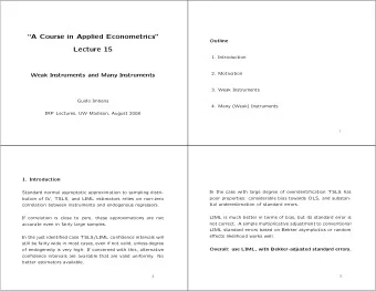
A Course in Applied Econometrics 1. Introduction Lecture 13 2. - - PowerPoint PPT Presentation

▶

Feb 26, 2024 118 likes •227 views

Outline A Course in Applied Econometrics 1. Introduction Lecture 13 2. Basics Bayesian Inference 3. Bernstein-Von Mises Theorem 4. Markov-Chain-Monte-Carlo Methods Guido Imbens 5. Example: Demand Models with Unobs Heterog in Prefer.

SLIDE 1

“A Course in Applied Econometrics” Lecture 13

Bayesian Inference

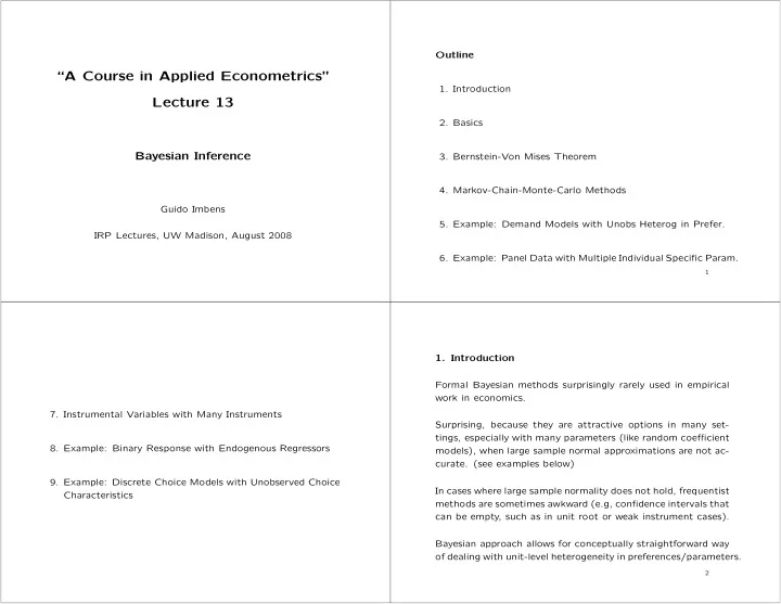
Guido Imbens IRP Lectures, UW Madison, August 2008 Outline

1. Introduction
2. Basics
3. Bernstein-Von Mises Theorem
4. Markov-Chain-Monte-Carlo Methods
5. Example: Demand Models with Unobs Heterog in Prefer.
6. Example: Panel Data with Multiple Individual Specific Param.

7. Instrumental Variables with Many Instruments
8. Example: Binary Response with Endogenous Regressors
9. Example: Discrete Choice Models with Unobserved Choice

Characteristics

1. Introduction

Formal Bayesian methods surprisingly rarely used in empirical work in economics. Surprising, because they are attractive options in many set- tings, especially with many parameters (like random coefficient models), when large sample normal approximations are not ac-

curate. (see examples below)

In cases where large sample normality does not hold, frequentist methods are sometimes awkward (e.g, confidence intervals that can be empty, such as in unit root or weak instrument cases). Bayesian approach allows for conceptually straightforward way

f dealing with unit-level heterogeneity in preferences/parameters.

SLIDE 2

Why are Bayesian methods not used more widely?

1. choice of methods does not matter (bernstein-von mises

theorem)

2. difficulty in specifying prior distribution (not “objective”)
3. need for fully parametric model
4. computational difficulties

2.A Basics: The General Case Model: fX|θ(x|θ). As a function of the parameter this is called the likelihood function, and denoted by L(θ|x). A prior distribution for the parameters, p(θ). The posterior distribution, p(θ|x) = fX,θ(x, θ) fX(x) = fX|θ(x|θ) · p(θ)

fX|θ(x|θ) · p(θ)dθ.

Note that, as a function of θ, the posterior is proportional to p(θ|x) ∝ fX|θ(x|θ) · p(θ) = L(θ|x) · p(θ).

2.B Example: The Normal Case Suppose the conditional distribution of X given the parameter µ is N(µ, 1). Suppose the prior distribution for µ to be N(0, 100). The posterior distribution is proportional to fµ|X(µ|x) ∝ exp

−1

2(x − µ)2

· exp
−

1 2 · 100µ2

= exp −1

2(x2 − 2xµ + µ2 + µ2/100) ∝ exp(− 1 2(100/101)(µ − (100/101)x)2) ∼ N(x · 100/101, 100/101)

2.B The Normal Case with General Normal Prior Distri- bution Model: N(µ, σ2) Prior distribution for µ is N(µ0, τ2). Then the posterior distribution is: fµ|X(µ|x) ∼ N

x/σ2 + µ0/τ2

1/σ2 + 1/τ2 , 1 1/τ2 + 1/σ2)

The result is quite intuitive: the posterior mean is a weighted average of the prior mean µ0 and the observation x with weights proportional to the precision, 1/σ2 for x and 1/τ2 for µ0: E[µ|X = x] =

x σ2 + µ0 τ2 1 σ2 + 1 τ2

1 V(µ|X) = 1 σ2 + 1 τ2.

SLIDE 3

Suppose we are really sure about the value of µ before we conduct the experiment. In that case we would set τ2 small and the weight given to the observation would be small, and the posterior distribution would be close to the prior distribution. Suppose on the other hand we are very unsure about the value

f µ.

What value for τ should we choose? We can let τ go to infinity. Even though the prior distribution is not a proper distribution anymore if τ2 = ∞, the posterior distribution is perfectly well defined, namely µ|X ∼ N(X, σ2). In that case we have an improper prior distribution. We give equal prior weight to any value of µ (flat prior). That would seem to capture pretty well the idea that a priori we are ignorant about µ. This is not always easy to do. For example, a flat prior distri- bution is not always uninformative about particular functions

f parameters.

2.C The Normal Case with Multiple Observations N independent draws from N(µ, σ2), σ2 known. Prior distribution on µ is N(µ0, τ2). The likelihood function is L(µ|σ2, x1, . . . , xN) =

N

1 √ 2πσ2 exp

− 1

2σ2(xi − µ)2

Then µ|X1, . . . , XN ∼ N

x ·

1 1 + σ2/(N · τ2) + µ0 · σ2/(Nτ2) 1 + σ2/(Nτ2), σ2/N 1 + σ2/(Nτ2)

3.A Bernstein-Von Mises Theorem: normal example When N is large √ N(¯ x − µ)|x1, . . . , xN ≈ N(0, σ2). In large samples the prior does not matter. Moreover, in a frequentist analysis, in large samples, √ N(¯ x − µ)|µ ∼ N(0, σ2). Bayesian probability and frequentiest confidence intervals agree: Pr

µ ∈
X − 1.96 ·

σ √ N , X − 1.96 · σ √ N

X1, . . . , XN
≈ Pr
µ ∈
X − 1.96 ·

σ √ N , X − 1.96 · σ √ N

µ
≈ 0.95;

3.B Bernstein-Von Mises Theorem: general case This is known as the Bernstein-von Mises Theorem. Here is a general statement for the scalar case. Let the information matrix Iθ at θ: Iθ = −E

∂2

∂θ∂θ′ ln fX(x|θ)

= −
∂2

∂θ∂θ′ ln fX(x|θ)fX(x|θ)dx, and let σ2 = I−1

θ0 .

Let p(θ) be the prior distribution, and pθ|X1,...,XN(θ|X1, . . . , XN) be the posterior distribution. Now let us look at the distribution of a transformation of θ, γ = √ N(θ − θ0), with density pγ|X1,...,XN(γ|X1, . . . , XN) = pθ|X1,...,XN(θ0 + √ N · γ|X1, . . . , XN)/ √ N.

SLIDE 4

Now let us look at the posterior distribution for γ if in fact the data were generated by f(x|θ) with θ = θ0. In that case the posterior distribution of γ converges to a normal distribution with mean zero and variance equal to σ2 in the sense that sup

γ

pγ|X1,...,XN(γ|X1, . . . , XN) −

1 √ 2πσ2 exp

− 1

2σ2γ2

→ 0. See Van der Vaart (2001), or Ferguson (1996).

At the same time, if the true value is θ0, then the mle ˆ θmle also has a limiting distribution with mean zero and variance σ2: √ N(ˆ θml − θ0)

d

− → N(0, σ2). The implication is that we can interpret confidence intervals as approximate probability intervals from a Bayesian perspective. Specifically, let the 95% confidence interval be [ˆ θml − 1.96 · ˆ σ/ √ N, ˆ θml + 1.96 · ˆ σ/ √ N]. Then, approximately, Pr

θml − 1.96 · ˆ σ/ √ N ≤ θ ≤ ˆ θml + 1.96 · ˆ σ/ √ N

X1, . . . , XN
−

→ 0.95.

3.C When Bernstein-Von Mises Fails There are important cases where this result does not hold, typ- ically when convergence to the limit distribution is not uniform. One is the unit-root setting. In a simple first order autore- gressive example it is still the case that with a normal prior distribution for the autoregressive parameter the posterior dis- tribution is normal (see Sims and Uhlig, 1991). However, if the true value of the autoregressive parameter is unity, the sampling distribution is not normal even in large samples. In such settings one has to take a more principled stand whether

ne wants to make subjective probability statements, or fre-

quentist claims.

4. Numerical Methods: Markov-Chain-Monte-Carlo

The general idea is to construct a chain, or sequence of values, θ0, θ1, . . . , such that for large k, θk can be viewed as a draw from the posterior distribution of θ given the data. This is implemented through an algorithm that, given a current value of the parameter vector θk, and given the data X1, . . . , XN draws a new value θk+1 from a distribution f(·) indexed by θk and the data: θk+1 ∼ f(θ|θk, data), in such a way that if the original θk came from the posterior distribution, then so does θk+1 θk|data ∼ p(θ|data), then θk+1|data ∼ p(θ|data).

SLIDE 5

In many cases, irrespective of where we start, that is, irrespec- tive of θ0, as k − → ∞, it will be the case that the distribution

f the parameter conditional only on the data converges to the

posterior distributionas k − → ∞: θk|data

d

− → p(θ|data), Then just pick a θ0 and approximate the mean and standard deviation of the posterior distribution as ˆ E[θ|data] = 1 K − K0 + 1

K

k=K0

θk, ˆ V[θ|data] = 1 K − K0 + 1

K

k=K0
θk − ˆ

E[θ|data]

2 .

The first K0 − 1 iterations are discarded to let algorithm con- verge to the stationary distribution, or “burn in.”

4.A Gibbs Sampling The idea being the Gibbs sampler is to partition the vector of parameters θ into two (or more) parts, θ′ = (θ′

1, θ′ 2). Instead of

sampling θk+1 directly from a conditional distribution of f(θ|θk, data), it may be easier to sample θ1,k+1 from the conditional distri- bution p(θ1|θ2,k, data), and then sample θ2,k+1 from p(θ2|θ1,k+1, data). It is clear that if (θ1,k, θ2,k) is from the posterior distribution, then so is (θ1,k, θ2,k).

4.B Data Augmentation Suppose we are interested in estimating the parameters of a censored regression or Tobit model. There is a latent variable Y ∗

i = X′ iβ + εi,

εi|Xi ∼ N(0, 1) We observe Yi = max(0, Y ∗

i ),

and the regressors Xi. Suppose the prior distribution for β is normal with some mean µ, and some covariance matrix Ω.

The posterior distribution for β does not have a closed form expression. The first key insight is to view both the vector Y∗ = (Y ∗

1 , . . . , Y ∗ N) and β as unknown random variables.

The Gibbs sampler consists of two steps. First we draw all the missing elements of Y∗ given the current value of the parameter β, say βk Y ∗

i |β, data ∼ TN

X′

iβ, 1, 0

if observation i is truncated, where TN(µ, σ2, c) denotes a trun- cated normal distribution with mean µ, variance σ2, and trun- cation point c (truncated from above). Second, we draw a new value for the parameter, βk+1 given the data and given the (partly drawn) Y∗: p

β|data, Y∗ ∼ N

X′X + Ω−1−1 ·
X′Y + Ω−1µ
,
X′X + Ω−1−1

SLIDE 6

4.C Metropolis Hastings We are again interested in p(θ|data). In this case L(θ|data) is assumed to be easy to evaluate. Draw a new candidate value for the chain from a candidate distribution q(θ|θk, data). We will either accept the new value with probability The probability that the new draw θ is accepted is ρ(θk, θ) = min

1, p(θ|data) · q(θk|θ, data)

p(θk|data) · q(θ|θk, data)

so that Pr

θk+1 = θ
= ρ(θk, θ),

and Pr

θk+1 = θk
= 1 − ρ(θk, θ).

The optimal (typically infeasible) choice for the candidate dis- tribution is q∗(θ|θk, data) = p(θ|data) = ⇒ ρ(θk, θ) = 1

5. Example: Demand Models with Unobs Heterog in Prefer. Rossi, McCulloch, and Allenby (1996, RMA) are interested in the optimal design of coupon policies. Supermarkets can choose to offer identical coupons for a particular product. Alternatively, they may choose to offer differential coupons based on consumer’s fixed characteristics. Taking this ever further, they could tailoring the coupon value to the evidence for price sensitivity contained in purchase pat- terns. Need to allow for household-level heterogeneity in taste param- eters and price elasticities. Even with large amounts of data available, there will be many households for whom these pa- rameters cannot be estimated precisely. RMA therefore use a hieararchical, or random coefficients model.

RMA model households choosing the product with the highest utility, where utility for household i, product j, j = 0, 1, . . . , J, at purchase time t is Uijt = X′

itβi + ǫijt,

with the ǫijt independent accross households, products and purchase times, and normally distributed with product-specific variances σ2

j (and σ2 0 normalized to one).

The Xit are observed choice characteristics that in the RMA application include price, some marketing variables, as well as brand dummies. All choice characteristics are assumed to be exogenous, al- though that assumption may be questioned for the price and marketing variables.

Because for some households we have few purchases, it is not possible to accurately estimate all βi parameters. RMA there- fore assume that the household-specific taste parameters are random draws from a normal distribution centered at Z′

iΓ:

βi = Z′

iΓ + ηi,

ηi ∼ N(0, Σ). Now Gibbs sampling can be used to obtain draws from the posterior distribution of the βi.

SLIDE 7

The first step is to draw the household parameters βi given the utilities Uijt and the common parameters Γ, Σ, and σ2

j . This

is straightforward, because we have a standard normal linear model for the utilities, with a normal prior distribution for βi with parameters Z′

iΓ and variance Σ, and Ti observations. We

can draw from this posterior distribution for each household i. In the second step we draw the σ2

j using the results for the

normal distribution with known mean and unknown variance. The third step is to draw from the posterior of Γ and Σ, given the βi. This again is just a normal linear model, now with unknown mean and unknown variance. The fourth step is to draw the unobserved utilities given the βi and the data. Doing this one household/choice at a time, conditioning on the utilities for the other choices, this merely involves drawing from a truncated normal distribution, which is simple and fast.

6. Example: Panel Data with Multiple Individual Specific

Param. Chamberlain and Hirano are interested in deriving predictive distributions for earnings using longitudinal data, using the model Yit = X′

iβ + Vit + αi + Uit/hi.

The second component in the model, Vit, is a first order au- toregressive component, Vit = γ · Vit−1 + Wit, Vi1 ∼ N(0, σ2

v ),

Wit ∼ N(0, σ2

w).

Uit ∼ N(0, 1).

Analyzing this model by attempting to estimate the αi and hi directly would be misguided. From a Bayesian perspective this corresponds to assuming a flat prior distribution on a high- dimensional parameter space. To avoid such pitfalls CH model αi and hi through a random effects specification. αi ∼ N(0, σ2

α).

and hi ∼ G(m/2, τ/2).

In their empirical application using data from the Panel Study

f Income Dynamics (PSID), CH find strong evidence of het-

erogeneity in conditional variances. quantiles of the predictive dist. of 1/ √ hi Quantile Sample 0.05 0.10 0.25 0.50 0.75 0.90 0.95 All (N=813) 0.04 0.05 0.07 0.11 0.20 0.45 0.81 HS Dropouts (N=37) 0.06 0.08 0.11 0.16 0.27 0.49 0.79 HS Grads (N=100) 0.04 0.05 0.06 0.11 0.21 0.49 0.93 C Grads (N=122) 0.03 0.04 0.05 0.09 0.18 0.40 0.75

SLIDE 8

However, CH wish to go beyond this and infer individual-level predictive distributions for earnings. Taking a particular individual, one can derive the posterior dis- tribution of αi, hi, β, σ2

v , and σ2 w, given that individual’s earnings

as well as other earnings, and predict future earnings. 0.90-0.10 quantile individual sample std 1 year out 5 years out 321 0.07 0.32 0.60 415 0.47 1.29 1.29 The variation reported in the CH results may have substantial importance for variation in optimal savings behavior by individ- uals.

7. Example: Instrumental Variables with Many Instru- ments Chamberlain and Imbens analyze the many instrument prob- lem from a Bayesian perspective. Reduced form for years of education, Xi = π0 + Z′

iπ1 + ηi,

combined with a linear specification for log earnings, Yi = α + β · Z′

iπ1 + εi.

CI assume joint normality for the reduced form errors,

ηi

∼ N(0, Ω).

This gives a likelihood function L(β, α, π0, π1, Ω|data). The focus of the CI paper is on inference for β, and the sen- sitivity of such inferences to the choice of prior distribution in settings with large numbers of instruments. A flat prior distribution may be a poor choice. One way to illustrate see this is that a flat prior on π1 leads to a prior on the sum K

k=1 π2 ik that puts most probability mass away from

zero. CI then show that the posterior distribution for β, under a flat prior distribution for π1 provides an accurate approximation to the sampling distribution of the TSLS estimator.

As an alternative CI suggest a hierarchical prior distribution with π1k ∼ N(µπ, σ2

π).

In the Angrist-Krueger 1991 compulsory schooling example there is in fact a substantive reason to believe that σ2

π is small

rather than the σ2

π = ∞ implicit in TSLS. If the π1k represent

the effect of the differences in the amount of required school- ing, one would expect the magnitude of the π1k to be less than the amount of variation in the compulsory schooling implying the standard deviation of the first stage coefficients should not be more than

1/12 = 0.289.

Using the Angrist-Krueger data CI find that the posterior dis- tribution for σπ is concentrated close to zero, with the posterior mean and median equal to 0.119.

SLIDE 9

8. Example: Binary Response with Endogenous Regres-

sors Geweke, Gowrisankaran, and Town are interested in estimating the effect of hospital quality on mortality, taking into account possibly non-random selection of patients into hospitals. Pa- tients can choose from 114 hospitals. Given their characteris- tics Zi, latent mortality is Y ∗

i = 114

Cijβj + Z′

iγ + ǫi,

where Cij is an indicator for patient i going to hospital j. The focus is on the hospital effects on mortality, βj. Realized mor- tality is Yi = 1{Y ∗

i ≥ 0}.

The concern is about selection into the hospitals, and the pos- sibility that this is related to unobserved components of latent mortality GGT model latent the latent utility for patient i as- sociated with hospital j as C∗

ij = X′ ijα + ηij,

where the Xij are hospital-individual specific characteristics, including distance to hospital. Patient i then chooses hospital j if C∗

ij ≥ Cik,

for k = 1, . . . , 114.

The endogeneity is modelled through the potential correlation between ηij and ǫi. Specifically, GGT asssume that as ǫi =

114 ηij · δj + ζi, where the ζi is a standard normal random variable, independent

f the other unobserved components.

GGT model the ηij as standard normal, independent across hospitals and across individuals. This is a very strong assump- tion, implying essentially the independence of irrelevant alter- natives property. One may wish to relax this by allowing for random coefficients on the hospital characteristics.

Given these modelling decisions GGT have a fully specified joint distribution of hospital choice and mortality given hospital and individual characteristics. The log likelihood function is highly nonlinear, and it is unlikely it can be well approximated by a quadratic function. GGT therefore use Bayesian methods, and in particular the Gibbs sampler to obtain draws from the posterior distribution

f interest.

In their empirical analysis GGT find strong evidence for non- random selection. They find that higher quality hospitals at- tract sicker patients, to the extent that a model based on exogenous selection would have led to misleading conclusions

n hospital quality.

SLIDE 10

9. Example: Discrete Choice Models with Unobserved Choice Characteristics Athey and Imbens (2007, AI) study discrete choice models, allowing both for unobserved individual heterogeneity in taste parameters as well as for multiple unobserved choice charac- teristics. In such settings the likelihood function is multi-modal, and frequentist approximations based on quadratic approximations to the log likelihood function around the maximum likelihood estimator are unlikely to be accurate.

The specific model AI use assumes that the utility for individual i in market t for choice j is Uijt = X′

itβi + ξ′ jγi + ǫijt,

where Xit are market-specific observed choice characteristics, ξj is a vector of unobserved choice characteristics, and ǫijt is an idiosyncratic error term, with a normal distribution centered at zero, and with the variance normalized to unity. The individual-specific taste parameters for both the observed and unobserved choice characteristics normally distributed:

γi

|Zi ∼ N(∆Zi, Ω),

with the Zi observed individual characteristics.

AI specify a prior distribution on the common parameters, ∆, and Ω, and on the values of the unobserved choice character- istics ξj. Using mcmc with the unobserved utilities as unobserved ran- dom variables makes sampling from the posterior distribution conceptually straightforward even in cases with more than one unobserved choice characteristic. In contrast, earlier studies using multiple unobserved choice characteristics (Elrod and Keane, 1995; Goettler and Shachar, 2001), using frequentist methods, faced much heavier compu- tational burdens.