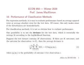
ECON 950 Winter 2020 Prof. James MacKinnon 9. Going Beyond Linear - PowerPoint PPT Presentation
ECON 950 Winter 2020 Prof. James MacKinnon 9. Going Beyond Linear Models Linear regression, linear discriminant analysis, and logistic regression all rely on models that are linear in the inputs. We often need to go beyond such models. The
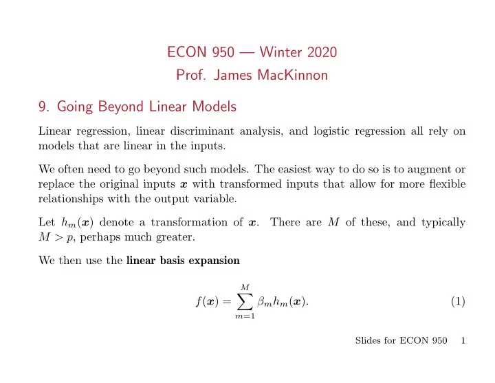
ECON 950 — Winter 2020 Prof. James MacKinnon 9. Going Beyond Linear Models Linear regression, linear discriminant analysis, and logistic regression all rely on models that are linear in the inputs. We often need to go beyond such models. The easiest way to do so is to augment or replace the original inputs x with transformed inputs that allow for more flexible relationships with the output variable. Let h m ( x ) denote a transformation of x . There are M of these, and typically M > p , perhaps much greater. We then use the linear basis expansion ∑ M f ( x ) = β m h m ( x ) . (1) m =1 Slides for ECON 950 1
Once we have chosen the basis expansion, we can fit all sorts of models just as we did before. In particular, we can use ordinary linear regression or logistic regression, perhaps with L 1 , L 2 , elastic-net, or some fancier form of regularization. • If h m ( x ) = x m , m = 1 , . . . , p with M = p , we get the original linear model. • If h m ( x ) = x 2 j and/or x j x k for m > p , we can augment the original model with polynomial and/or cross-product terms. Unfortunately, a full polynomial model of degree d requires O ( p d ) terms. When d = 2, we have p linear terms, p quadratic terms, and p ∗ ( p − 1) / 2 cross-product terms. Global polynomials do not work very well. It is much better to use piecewise polynomials and splines which allow for local polynomial representations. • We can use transformations of single inputs, such as h m ( x ) = log( x j ) or √ x j , either replacing x j or as additional regressors. • We can use functions of several inputs, such as h ( x ) = || x || . Slides for ECON 950 2
• We can create all sorts of indicator (dummy) variables, such as h m ( x ) = I ( l m ≤ x k < u m ). In such cases, we often create a lot of them. For example, we could divide the range of x k into M k nonoverlapping segments. The M k dummies that result would allow a piecewise constant relationship between x k and y . In such a case, it would often be a very good idea to use a form of L 2 regular- ization, not shrinking the coefficients towards zero, but instead shrinking their first differences, as in Shiller (1973) and Gersovitz and MacKinnon (1978). To avoid estimating too many coefficients, we often have to impose restrictions. One popular one is additivity : p p ∑ ∑ ∑ M f ( x ) = f j ( x j ) = β jm h jm ( x j ) . (2) j =1 j =1 m =1 In many cases, it is important to employ selection methods, such as the (possibly grouped) lasso. It is also often important to use regularization, including lasso, ridge, and other methods to be discussed. Slides for ECON 950 3
9.1. Piecewise Polynomials and Splines A piecewise polynomial function f ( x ) simply divides the domain of x (assumed one-dimensional for now) into continguous intervals. In the simplest case, with M = 3, h 1 ( x ) = I ( x ≤ ξ 1 ) , h 2 ( x ) = I ( ξ 1 < x ≤ ξ 2 ) , h 3 ( x ) = I ( ξ 2 < x ) . (3) Thus, for this piecewise constant function, 3 ∑ f ( x ) = β m h m ( x ) . (4) m =1 The least squares estimates are just 1 ˆ y ⊤ h m , β m = ¯ y m = (5) ι ⊤ h m where h m is a vector with typical element h m ( x i ). It is a vector of 0s and 1s. Slides for ECON 950 4
Of course, a piecewise constant function is pretty silly; see the upper left panel of ESL-fig5.01.pdf. A less stupid approximation is piecewise linear . Now we have six basis functions when there are three regions. Numbers 4 to 6 are h 1 ( x ) x, h 2 ( x ) x, and h 3 ( x ) x. (6) But f ( x ) still has gaps in it; see the upper right panel of ESL-fig5.01.pdf. The best way to avoid gaps is to constrain the basis functions to meet at ξ 1 and ξ 2 , which are called knots . This is most easily accomplished by using regression splines . In the linear case with three regions, there are four basis functions: h 1 ( x ) = 1 , h 2 ( x ) = x, h 3 ( x ) = ( x − ξ 1 ) + , h 4 ( x ) = ( x − ξ 2 ) + . (7) See the lower left panel of ESL-fig5.01.pdf. h 3 ( x ) is plotted the lower right panel. Here h 3 ( x ) and h 4 ( x ) are truncated power basis functions . Linear functions are pretty restrictive. Slides for ECON 950 5
It is very common to use a cubic spline , which is constrained to be continuous and to have continuous first and second derivatives. With three regions (and therefore two knots) a cubic spline has six basis functions. These are h 3 ( x ) = x 2 , h 4 ( x ) = x 3 , h 1 ( x ) = 1 , h 2 ( x ) = x, (8) h 5 ( x ) = ( x − ξ 1 ) 3 h 6 ( x ) = ( x − ξ 2 ) 3 + , + . In general, a spline is of order M and has K knots. Thus (7) is an order-2 spline with 2 knots, and (8) is an order-4 spline that also has 2 knots. The basis functions for an order- M spline with K knots ξ k are: h j ( x ) = x j − 1 , j = 1 , . . . , M, (9) h M + k ( x ) = ( x − ξ k ) M − 1 , k = 1 , . . . , K. (10) + In practice, M = 1 , 2 , 4. For some reason, cubic splines are much more popular than quadratic ones. For computational reasons when N and K are large, it is desirable to use B -splines rather than ordinary ones. See the Appendix to Chapter 5 of ESL. Slides for ECON 950 6
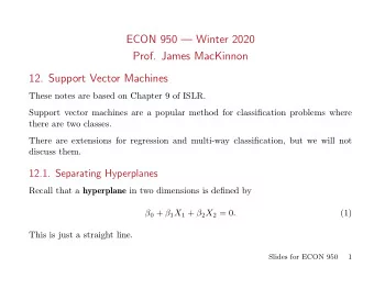
9.2. Natural Cubic Splines Polynomials tend to behave badly near boundaries. Using them to extrapolate is extremely dangerous. A natural cubic spline adds additional constraints, namely, that the function is linear beyond the boundary knots. This saves four degrees of freedom (2 at each boundary knot) and reduces variance, at the expense of higher bias. The freed degrees of freedom can be used to add additional interior knots. In general, a cubic spline with K knots can be represented as 3 K ∑ ∑ β j x j + θ k ( x − ξ k ) 3 f ( x ) = + ; (11) j =0 k =1 compare (8). The boundary conditions imply that K K ∑ ∑ β 2 = β 3 = 0 , θ k = 0 , ξ k θ k = 0 . (12) k =1 k =1 Slides for ECON 950 7
Combining these with (11) gives us the basis functions for the natural cubic spline with K knots. Instead of K + 4 basis functions, there will be just K . The first two basis functions are just 1 and x . The remaining K − 2 are N k +2 ( x ) = ( x − ξ k ) 3 + − ( x − ξ K ) 3 − ( x − ξ K − 1 ) 3 + − ( x − ξ K ) 3 + + (13) ξ K − ξ k ξ K − ξ K − 1 for k = 1 , . . . , K − 2. Since the number of basis functions is only K , we may be able to have quite a few knots. When there are two or more inputs, they cannot both include a constant among the basis functions. ESL discusses a heart-disease dataset. For the continuous regressors, they use natural cubic splines with 3 interior knots. ESL fits a logistic regression model, without regularization, using backwards step deletion. Slides for ECON 950 8
ESL drops terms, not individual regressors, using AIC. Only the alcohol term is actually dropped. The final model has one binary variable and five continuous ones. Each of the latter uses a natural spline with 3 interior knots. There are 22 coefficients (a constant, a family history dummy, and five splines with 4 each). ESL-fig5.04.pdf plots the fitted natural-spline functions along with pointwise bands of width two standard errors. Let θ denote the entire vector of parameters, and ˆ θ its ML estimator. Then Var(ˆ � θ ) = ˆ Σ is computed by the usual formula for logistic regression: ( ) − 1 , Var(ˆ � X ⊤ Υ (ˆ θ ) = θ ) X (14) where λ 2 ( X t θ ) ( ) . Υ t ( θ ) ≡ (15) Λ ( X t θ ) 1 − Λ ( X t θ ) Slides for ECON 950 9
Here Λ ( · ) is the logistic function, and λ ( · ) is its derivative. That is, e x 1 Λ( x ) ≡ 1 + e − x = (16) 1 + e x e x λ ( x ) ≡ (1 + e x ) 2 = Λ( x )Λ( − x ) . (17) Then the pointwise standard errors are the square roots of ( ˆ ) = h j ( x ji ) ⊤ ˆ � Var f ( x ji ) Σ jj h j ( x ji ) , (18) where x ji is the value of the j th variable for observation i , and h j ( x ji ) is the vector of values of the basis functions for x ji . In this case, it is a 4- -vector. Notice how the confidence bands are wide where the data are sparse and narrow where they are dense. Notice the unexpected shapes of the curves for sbp (systolic blood pressure) and obesity (BMI). These are retrospective data! Slides for ECON 950 10
9.3. Smoothing Splines Consider the minimization problem ( N ) ∫ ( ∑ ( ) 2 + λ ) 2 dt f ′′ ( t ) min ( y i − f ( x i , λ ) , (19) f i =1 where λ is a fixed smoothing parameter. When λ = ∞ , minimizing (19) yields the OLS estimates, since the second derivative must be 0. When λ = 0, minimizing (19) yields a perfect fit, provided every x i is unique, because f ( x ) can be any function that goes through every data point. It can be shown (see Exercise 5.7, which is nontrivial) that the minimizer is a natural cubic spline with knots at all of the (unique) x i . The penalty term shrinks the spline coefficients towards the least squares fit. We can write the solution as N ∑ f ( x ) = θ j N j ( x ) , (20) j =1 Slides for ECON 950 11
Recommend
More recommend
Explore More Topics
Stay informed with curated content and fresh updates.
