Introduction to Machine Learning 3. Instance Based Learning Alex - PowerPoint PPT Presentation
Introduction to Machine Learning 3. Instance Based Learning Alex Smola Carnegie Mellon University http://alex.smola.org/teaching/cmu2013-10-701 10-701 Outline Parzen Windows Kernels, algorithm Model selection Crossvalidation, leave
Introduction to Machine Learning 3. Instance Based Learning Alex Smola Carnegie Mellon University http://alex.smola.org/teaching/cmu2013-10-701 10-701
Outline • Parzen Windows Kernels, algorithm • Model selection Crossvalidation, leave one out, bias variance • Watson-Nadaraya estimator Classification, regression, novelty detection • Nearest Neighbor estimator Limit case of Parzen Windows
Parzen Windows Parzen
Density Estimation • Observe some data x i • Want to estimate p(x) • Find unusual observations (e.g. security) • Find typical observations (e.g. prototypes) • Classifier via Bayes Rule p ( y | x ) = p ( x, y ) p ( x | y ) p ( y ) = p ( x ) P y 0 p ( x | y 0 ) p ( y 0 ) • Need tool for computing p(x) easily
Bin Counting • Discrete random variables, e.g. • English, Chinese, German, French, ... • Male, Female • Bin counting (record # of occurrences) 25 English Chinese German French Spanish male 5 2 3 1 0 female 6 3 2 2 1
Bin Counting • Discrete random variables, e.g. • English, Chinese, German, French, ... • Male, Female • Bin counting (record # of occurrences) 25 English Chinese German French Spanish male 0.2 0.08 0.12 0.04 0 female 0.24 0.12 0.08 0.08 0.04
Bin Counting • Discrete random variables, e.g. • English, Chinese, German, French, ... • Male, Female • Bin counting (record # of occurrences) 25 English Chinese German French Spanish male 0.2 0.08 0.12 0.04 0 female 0.24 0.12 0.08 0.08 0.04
Bin Counting • Discrete random variables, e.g. • English, Chinese, German, French, ... • Male, Female not enough data • Bin counting (record # of occurrences) 25 English Chinese German French Spanish male 0.2 0.08 0.12 0.04 0 female 0.24 0.12 0.08 0.08 0.04
Curse of dimensionality (lite) • Discrete random variables, e.g. • English, Chinese, German, French, ... • Male, Female #bins grows • ZIP code exponentially • Day of the week • Operating system • ... • Continuous random variables • Income need many bins • Bandwidth per dimension • Time
Curse of dimensionality (lite) • Discrete random variables, e.g. • English, Chinese, German, French, ... • Male, Female #bins grows • ZIP code exponentially • Day of the week • Operating system • ... • Continuous random variables • Income need many bins • Bandwidth per dimension • Time
Density Estimation 0.10 0.05 sample underlying density 0.04 0.03 0.05 0.02 0.01 0.00 0.00 40 50 60 70 80 90 100 110 40 50 60 70 80 90 100 110 • Continuous domain = infinite number of bins • Curse of dimensionality • 10 bins on [0, 1] is probably good • 10 10 bins on [0, 1] 10 requires high accuracy in estimate: probability mass per cell also decreases by 10 10 .
Bin Counting
Bin Counting
Bin Counting
Bin Counting can’t we just go and smooth this out?
What is happening? • Hoeffding’s theorem (� � ) m � E [ x ] − 1 � � ≤ 2 e − 2 m ✏ 2 X Pr � � x i � > ✏ � � m i =1 For any average of [0,1] iid random variables. • Bin counting • Random variables x i are events in bins • Apply Hoeffding’s theorem to each bin • Take the union bound over all bins to guarantee that all estimates converge
Density Estimation • Hoeffding’s theorem (� � ) m � E [ x ] − 1 � � ≤ 2 e − 2 m ✏ 2 X Pr � � x i � > ✏ � � m i =1 • Applying the union bound and Hoeffding ✓ ◆ X Pr sup | ˆ p ( a ) − p ( a ) | ≥ ✏ Pr ( | ˆ p ( a ) − p ( a ) | ≥ ✏ ) ≤ a ∈ A a ∈ A − 2 m ✏ 2 � � ≤ 2 | A | exp good news • Solving for error probability r log 2 | A | − log � � 2 | A | ≤ exp( − m ✏ 2 ) = ⇒ ✏ ≤ 2 m
Density Estimation • Hoeffding’s theorem (� � ) m � E [ x ] − 1 � � ≤ 2 e − 2 m ✏ 2 X Pr � � x i � > ✏ � � m i =1 • Applying the union bound and Hoeffding ✓ ◆ X Pr sup | ˆ p ( a ) − p ( a ) | ≥ ✏ Pr ( | ˆ p ( a ) − p ( a ) | ≥ ✏ ) ≤ a ∈ A a ∈ A but not good − 2 m ✏ 2 � � ≤ 2 | A | exp enough good news • Solving for error probability r log 2 | A | − log � � 2 | A | ≤ exp( − m ✏ 2 ) = ⇒ ✏ ≤ 2 m
Density Estimation • Hoeffding’s theorem (� � ) m � E [ x ] − 1 � � ≤ 2 e − 2 m ✏ 2 X Pr � � x i � > ✏ � � m bins not i =1 • Applying the union bound and Hoeffding independent ✓ ◆ X Pr sup | ˆ p ( a ) − p ( a ) | ≥ ✏ Pr ( | ˆ p ( a ) − p ( a ) | ≥ ✏ ) ≤ a ∈ A a ∈ A but not good − 2 m ✏ 2 � � ≤ 2 | A | exp enough good news • Solving for error probability r log 2 | A | − log � � 2 | A | ≤ exp( − m ✏ 2 ) = ⇒ ✏ ≤ 2 m
Bin Counting
Bin Counting can’t we just go and smooth this out?
Parzen Windows • Naive approach Use empirical density (delta distributions) m p emp ( x ) = 1 X δ x i ( x ) m i =1 • This breaks if we see slightly different instances • Kernel density estimate Smear out empirical density with a nonnegative smoothing kernel k x (x’) satisfying Z k x ( x 0 ) dx 0 = 1 for all x X
Parzen Windows • Density estimate m p emp ( x ) = 1 X δ x i ( x ) m i =1 m p ( x ) = 1 X ˆ k x i ( x ) m • Smoothing kernels i =1 1.0 1.0 1.0 1.0 Gauss Epanechikov Uniform Laplace 0.5 0.5 0.5 0.5 0.0 0.0 0.0 0.0 -2 -1 0 1 2 -2 -1 0 1 2 -2 -1 0 1 2 -2 -1 0 1 2 3 1 1 2 x 2 (2 π ) − 1 2 e − 1 2 e − | x | 4 max(0 , 1 − x 2 ) 2 χ [ − 1 , 1] ( x )
Smoothing
Smoothing dist = norm(X - x * ones(1,m),'columns'); p = (1/m) * ((2 * pi)**(-d/2)) * sum(exp(-0.5 * dist.**2))
Smoothing
Smoothing
Size matters 0.050 0.050 0.050 0.050 0.025 0.025 0.025 0.025 0.000 0.000 0.000 0.000 40 60 80 100 40 60 80 100 40 60 80 100 40 60 80 100 0.3 1 3 10 0.10 0.05 0.04 0.03 0.05 0.02 0.01 0.00 0.00 40 50 60 70 80 90 100 110 40 50 60 70 80 90 100 110
Size matters Shape matters mostly in theory 0.050 0.050 0.050 0.050 0.025 0.025 0.025 0.025 0.000 0.000 0.000 0.000 40 60 80 100 40 60 80 100 40 60 80 100 40 60 80 100 ✓ x − x i ◆ • Kernel width k x i ( x ) = r − d h r • Too narrow overfits • Too wide smoothes with constant distribution • How to choose?
Model Selection
Maximum Likelihood • Need to measure how well we do • For density estimation we care about m Y Pr { X } = p ( x i ) i =1 • Finding a that maximizes P(X) will peak at all data points since x i explains x i best ... • Maxima are delta functions on data. • Overfitting!
Overfitting 0.050 Likelihood on training set is 0.025 0.025 much higher than typical. 0.000 40 60 80 100
Overfitting 0.050 density ≫ 0 Likelihood on training set is 0.025 0.025 much higher than typical. density 0 0.000 40 60 80 100
Underfitting 0.050 Likelihood on training set is very similar to 0.025 typical one. Too simple. 0.000 40 60 80 100
Model Selection • Validation • Use some of the data to estimate density. • Use other part to evaluate how well it works • Pick the parameter that works best n 0 L ( X 0 | X ) := 1 X p ( x 0 log ˆ i ) n 0 i =1 • Learning Theory • Use data to build model • Measure complexity and use this to bound n 1 X log ˆ p ( x i ) − E x [log ˆ p ( x )] n i =1
Model Selection • Validation • Use some of the data to estimate density. • Use other part to evaluate how well it works easy • Pick the parameter that works best n 0 L ( X 0 | X ) := 1 X p ( x 0 log ˆ i ) n 0 i =1 • Learning Theory • Use data to build model • Measure complexity and use this to bound n 1 X log ˆ p ( x i ) − E x [log ˆ p ( x )] n i =1
Model Selection • Validation • Use some of the data to estimate density. • Use other part to evaluate how well it works easy • Pick the parameter that works best n 0 L ( X 0 | X ) := 1 X p ( x 0 log ˆ i ) n 0 i =1 wasteful • Learning Theory • Use data to build model • Measure complexity and use this to bound n 1 X log ˆ p ( x i ) − E x [log ˆ p ( x )] n i =1
Model Selection • Validation • Use some of the data to estimate density. • Use other part to evaluate how well it works easy • Pick the parameter that works best n 0 L ( X 0 | X ) := 1 X p ( x 0 log ˆ i ) n 0 i =1 wasteful • Learning Theory • Use data to build model • Measure complexity and use this to bound n 1 difficult X log ˆ p ( x i ) − E x [log ˆ p ( x )] n i =1
Model Selection • Leave-one-out Crossvalidation • Use almost all data to estimate density. • Use single instance to estimate how well it works 1 X log p ( x i | X \ x i ) = log k ( x i , x j ) n − 1 j 6 = i • This has huge variance • Average over estimates for all training data • Pick the parameter that works best • Simple implementation n n � 1 1 where p ( x ) = 1 n X X log n − 1 p ( x i ) − n − 1 k ( x i , x i ) k ( x i , x ) n n i =1 i =1
Leave-one out estimate
Optimal estimate
Recommend
More recommend
Explore More Topics
Stay informed with curated content and fresh updates.


