The Distributional Dynamics of Income, Earnings and Consumption JAE - PowerPoint PPT Presentation
The Distributional Dynamics of Income, Earnings and Consumption JAE Lectures CEMFI, Madrid June 6-7 2008 Richard Blundell University College London and Institute for Fiscal Studies Setting the Scene I Inequality has many linked dimensions:
The Distributional Dynamics of Income, Earnings and Consumption JAE Lectures CEMFI, Madrid June 6-7 2008 Richard Blundell University College London and Institute for Fiscal Studies
Setting the Scene I Inequality has many linked dimensions: wages, incomes and consumption I The link between the various types of inequality is mediated by multiple insurance mechanisms I including labour supply, taxation, consumption smoothing, informal mechanisms, etc I Wages I earnings I joint earnings I income I consumption � hours � Family labour supply � Taxes and transfers � Self-insurance/ partial-insurance/ advance information
`Insurance' mechanisms. . . I These mechanisms will vary in importance across different types of households at different points of their life-cycle and at different points in time. I The manner and scope for insurance depends on the durability of income shocks I The objective here is to understand the distributional dynamics of wages, earn- ings, income and consumption I That is to understand the transmission between wages, earnings, income and consumption inequality � 1980s in the US and UK have particularly interesting episodes, also Japan and Australia = >
These lectures are an attempt to reconcile three key literatures: I I. Examination of the evolution in inequality over time for consumption and income � In particular, studies from the BLS, Johnson and Smeeding (2005); early work in the US by Cutler and Katz (1992) and in the UK by Blundell and Preston (1991) and Atkinson (1997), etc - Table I
These lectures are an attempt to reconcile three key literatures: I I. Examination of inequality over time via consumption and income I II. Econometric work on the panel data decomposition of the income process � Lillard and Willis (1978), Lillard and Weiss (1979), MaCurdy(1982), Abowd and Card (1989), Gottschalk and Mof�tt (1995, 2004), Baker (1997), Dickens (2000), Haider (2001), Meghir and Pistaferri (2004), Browning, Ejrnaes and Alverez (2007), Haider and Solon (2006), etc econometric work on the panel data decomposition of income processes
These lectures are an attempt to reconcile three key literatures: I I. Examination of inequality over time via consumption and income I II. Econometric work on the panel data decomposition of the income process I II. Work on intertemporal decisions under uncertainty, especially on partial insur- ance, excess sensitivity: � Hall and Mishkin (1982), Campbell and Deaton (1989), Cochrane (1991), Deaton and Paxson (1994), Attanasio and Davis (1996), Blundell and Preston (1998), Krueger and Perri (2004, 2006), Heathcote et al (2005), Storresletten et al (2004), Attanasio and Pavoni (2006), Primiceri and Van Rens (2006), etc
These lectures are an attempt to reconcile three key literatures: I I. Examination of inequality over time via consumption and income I II. Econometric work on the panel data decomposition of the income process I III. Work on intertemporal decisions under uncertainty, especially on partial insur- ance, excess sensitivity: � Hall and Mishkin (1982), Campbell and Deaton (1989), Cochrane (1991), Deaton and Paxson (1994), Attanasio and Davis (1996), Blundell and Preston (1998), Krueger and Perri (2006), Heathcote et al (2005), Storresletten et al (2004), Attanasio and Pavoni (2006), Primiceri and Van Rens (2006), Blundell, Pistaferri and Preston, etc � Information and human capital: � Cuhna, Heckman and Navarro (2005, 2007), Guvenen (2006, Huggett et al (2007)
JAE Lecture I: I Distributional Dynamics of Income, Earnings and Consumption I Developing the Transmission Parameter or `Partial Insurance' approach: � What do we do? � What do we �nd? JAE Lecture II: I How well does the Partial Insurance approach work? � Robustness to alternative representations of the economy � Bewley economy, alternative economies - draw on simulation studies I Are there other key avenues for `insurance'? I What features need developing/generalising?
I Some resilient features of the distribution of consumption � Construct quantile-quantile (QQ) plots as well as histograms of the sample. � The QQ plot depicts the points f y ( i ) ; � + � � � 1 ( i n ) g for i = 1 ; :::; n . � Use robust estimates for location and scale parameters � and � : median M ( Y ) = � and the median absolute deviation MAD ( Y ) � M ( j Y � M ( Y ) j ) ' 0 : 6745 � � Kolmogorov-Smirnov tests: p-values by 10 ; 000 random samples generated under � 2 ) � , ^ N (^ skewness test based on: [ Q 1 � p ( Y ) � M ( Y )] � [ M ( Y ) � Q p ( Y )] ; Q 1 � p ( Y ) � Q p ( Y ) where Q � ( Y ) is the � -th percentile. kurtosis test based on: [ O 7 ( Y ) � O 5 ( Y )] + [ O 3 ( Y ) � O 1 ( Y )] ; O 6 ( Y ) � O 2 ( Y ) where O � ( Y ) is the � -th octile.
I Figure 2a-d, US; Figure 3a-c, UK. � Log normal distribution of equivalised consumption by cohort and time. I Gibrat's law over the life-cycle for consumption rather than income? � Extend the Deaton-Paxson JPE result on the variances of log consumption over the life-cycle � There are many alternative regularity conditions that will yield a CLT, they all require a uniform asymptotic negligibility condition (relating to existence of mo- ments) and a limit on the degree of dependence of observations over time such as alpha mixing. I Figure 4a-d
Income dynamics (1) General speci�cation for income dynamics for consumer i of age a in time period t: Write log income ln Y i;a;t as: y i;a;t = B 0 i;a;t f i + Z 0 i;a;t ' + y P i;a;t + y T (1) i;a;t I where y P it is a persistent process of income shocks which adds to the individual- speci�c trend (by age and time) B 0 i;a;t f i and where y P it is a transitory shock repre- sented by some low order MA process. I Allow variances (or factor loadings) of y P and y T to vary with cohort, time,.. I For any cohort, an interesting possible speci�cation for B 0 i;t f i is B 0 (2) i;t f i = p t f 1 i + f 0 i
I If y T i;t is represented by a MA( q ) q X � j " i;t � j with � 0 � 1 : (3) v it = j =0 I and y P it by y P it = �y P (4) it � 1 + � it ; With q = 1 ; this implies a `key' quasi-difference moment restriction cov(� � y t ; � � y t � 2 ) = var( f 0 )(1 � � ) 2 + var( f 1 )� � p t � � p t � 2 � �� 1 var( " t � 2 ) (5) where � � = (1 � �L ) is the quasi-difference operator. I Note that for large � = 1 and small � 1 this implies (6) cov(� y t ; � y t � 2 ) ' var( f 1 )� p t � p t � 2 :
Idiosyncratic trends: I The term p t f 1 i could take a number of forms (a) deterministic idiosyncratic trend : p t f 1 i = r ( t ) f 1 i where r is known, e.g. r ( t ) = t (b) stochastic trend in `ability prices' : p t = p t � 1 + � t with E t � 1 � t = 0 I Evidence points to some periods of time where each is of key importance: � (a) early in working life (Solon et al.). Formally, this is a life-cycle effect. � (b) during periods of technical change when skill prices are changing across the unobserved ability distribution. Early 1980s in the US and UK, for example. For- mally, this is a calender time effect. I I will come back to look at various sensitivity results for � and p t f 1 i + f 0 i :
Income dynamics (2) I For each household i; I �rst consider a simple permanent-transitory decomposi- tion for log income: y it = Z 0 it ' + y P it + y T (7) it � with y P it = y P (8) it � 1 + � it � and transitory or mean-reverting component, y T it = v i;t q X � j " i;t � j with � 0 � 1 : (9) v it = j =0 I Implies a restrictive structure for the autocovariances of � y it (= � it + � v it ) ; where y it = log Y it � Z 0 it ':
Some (Simple) Empirics � How well does it work? � Tables III a, b and c present the autocovariance structure of the PSID and the BHPS (ECFP and JPID on my webpage). � this latent factor structure aligns `well' with the autocovariance structure of the PSID, the BHPS (UK), JPID(Japan) and the ECFP(Spain) � allows for general �xed effects and initial conditions. � regular deconvolution arguments lead to identi�cation of variances and com- plete distributions, e.g. Bonhomme and Robin (2006) � the key idea is to allow the variances (or loadings) of the factors to vary nonparametrically with cohort, education and time: - the relative variance of these factors is a measure of persistence or durability of labour income shocks.
Evolution of the Consumption Distribution - with Self-Insurance I At time t each individual i maximises the conditional expectation of a time sepa- rable, differentiable utility function: P T � t max C E t j =0 u ( C i;t + j ; Z i;t + j ) Z i;t + j incorporates taste shifters/non-separabilities and discount rate heterogeneity. � We set the retirement age at L , assumed known and certain, and the end of the life-cycle at T . We assume that there is no uncertainty about the date of death. � Individuals can self-insure using a simple credit market with access to a risk free bond with real return r t + j : Consumption and income are linked through the intertem- poral budget constraint A i;t + j +1 = (1 + r t + j ) ( A i;t + j + Y i;t + j � C i;t + j ) with A i;T = 0 :
Recommend
More recommend
Explore More Topics
Stay informed with curated content and fresh updates.
