ECON 950 Winter 2020 Prof. James MacKinnon 3. Methods Based on - PowerPoint PPT Presentation
ECON 950 Winter 2020 Prof. James MacKinnon 3. Methods Based on Linear Regression The methods discussed in this section are primarily intended for high-dimensional situations, where p is large relative to N , perhaps much larger than N . We
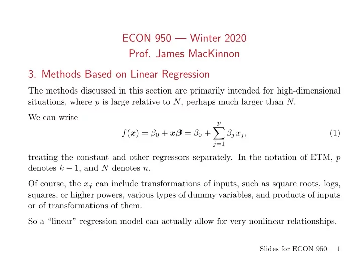
ECON 950 — Winter 2020 Prof. James MacKinnon 3. Methods Based on Linear Regression The methods discussed in this section are primarily intended for high-dimensional situations, where p is large relative to N , perhaps much larger than N . We can write p ∑ f ( x ) = β 0 + xβ = β 0 + β j x j , (1) j =1 treating the constant and other regressors separately. In the notation of ETM, p denotes k − 1, and N denotes n . Of course, the x j can include transformations of inputs, such as square roots, logs, squares, or higher powers, various types of dummy variables, and products of inputs or of transformations of them. So a “linear” regression model can actually allow for very nonlinear relationships. Slides for ECON 950 1
3.1. Regression by Successive Orthogonalization When the x j are orthogonal, the ˆ ⊤ y / x j ⊤ x j obtained by univariate regressions β j = x j of y on each of the x j are equal to the multiple regression least squares estimates. We can accomplish something similar even when the data are not orthogonal. This is called Gram-Schmidt Orthogonalization . It is related to the FWL Theorem. 1. Set z 0 = x 0 = ι . 2. Regress x 1 on z 0 to obtain a residual vector z 1 and coefficient ˆ γ 01 . 3. For j = 2 , . . . , p , regress x j on z 0 , . . . , z j − 1 to obtain a residual vector z j and coefficients ˆ γ ℓj for ℓ = 0 , . . . , j − 1. 4. Regress y on z p to obtain ˆ ⊤ y / z p ⊤ z p . β p = z p The scalar ˆ β p is the coefficient on x p in the multiple regression of y on a constant and all the x j . Note that step 3 simply involves j univariate regressions. If we did this p + 1 times, changing the ordering so that each of the x j came last, we could obtain all the OLS coefficients. Slides for ECON 950 2
The QR decomposition of X is X = ZD − 1 DΓ = QR , (2) where Z contains the columns z 0 to z p (in order), Γ is an upper triangular matrix containing the ˆ γ ℓj , and D is a diagonal matrix with typical diagonal element || z j || . Thus Q = ZD − 1 and R = DΓ . It can be seen that Q is an N × ( p + 1) orthogonal matrix with the property that Q ⊤ Q = I , and R is a ( p + 1) × ( p + 1) upper triangular matrix. The QR decomposition provides a convenient orthogonal basis for S ( X ). It is easy to see that ˆ β = ( X ⊤ X ) − 1 X ⊤ y = R − 1 Q ⊤ y , (3) because ( X ⊤ X ) − 1 = ( R ⊤ Q ⊤ QR ) − 1 = ( R ⊤ R ) − 1 = R − 1 ( R ⊤ ) − 1 , and X ⊤ y = R ⊤ Q ⊤ y . Slides for ECON 950 3
Since R is triangular, it is very easy to invert. Also, y = P X y = QQ ⊤ y . ˆ (4) so that SSR( ˆ β ) = ( y − QQ ⊤ y ) ⊤ ( y − QQ ⊤ y ) = y ⊤ y − y ⊤ QQ ⊤ y . (5) The diagonals of the hat matrix are the diagonals of QQ ⊤ . The QR decomposition is easy to implement and numerically stable. It requires O ( Np 2 ) operations. An alternative is to form X ⊤ X and X ⊤ y efficiently, use the Cholesky decomposition to invert X ⊤ X , and then multiply X ⊤ y by ( X ⊤ X ) − 1 . The Cholesky approach requires O ( p 3 + Np 2 / 2) operations. For p < < N , Cholesky wins, but for large p QR does. Never use a general matrix inversion routine, because such routines are not as stable as QR or Cholesky. In extreme cases, QR can yield reliable results when Cholesky does not. If X ⊤ X is not well-conditioned (i.e., if the ratio of the largest to the smallest eigenvalue is large), then it is much safer to use QR than Cholesky. Intelligent scaling helps. Slides for ECON 950 4
3.2. Subset Selection When p is large, OLS tends to have low bias but large variance. By setting some coefficients to zero, we can often reduce variance substantially while increasing bias only modestly. It can be hard to make sense of models with a great many coefficients. Best-subset regression tries every subset of size k = 1 , . . . , p to find the one that, for each k , has the smallest SSR. There is an efficient algorithm, but it becomes infeasible once p becomes even mod- erately large (say much over 40). Forward-stepwise selection and backward-stepwise selection are feasible even when p is large. The former works even if p > N . To begin the forward-stepwise selection procedure, we regress y on each of the x j and pick the one that yields the smallest SSR. Next, we add each of the remaining p − 1 regressors, one at a time, and pick the one that yields the smallest SSR. Slides for ECON 950 5
Then we add each of the remaining p − 2 regressors, one at a time, and pick the one that yields the smallest SSR. If we are using the QR decomposition, we can do this efficiently. We are just adding one more column to Z and hence Q , and one more row to Γ and hence R . We do this for each of the candidate regressors and calculate the SSR from (5) for each of them. We can reuse most of the elements of the old Q matrix. For backward-stepwise regression, we start with the full model (assuming that p < N ) and then successively drop regressors. At each step, we drop the one with the smallest t statistic. Smart stepwise programs will recognize that regressors often come in groups. It generally does not make sense to • Drop a regressor X if the model includes X 2 or XZ ; • Drop some dummy variables that are part of a set (e.g. some province dummies but not all, or some categorical dummies but not all). In cases like this, variables should be added, or subtracted, in groups. Slides for ECON 950 6
If we use either forward-stepwise or backward-stepwise selection, how do we decide which model to choose? The model with all p regressors will always fit best, in terms of SSR. We either need to penalize the number of parameters ( d ) or use cross-validation. 1 σ 2 ) = (1 + 2 d/N )ˆ σ 2 . C p : N (SSR + 2 d ˆ (6) σ 2 to SSR. Thus C p adds a penalty of 2 d ˆ The Akaike information criterion , or AIC , is defined for all models estimated by maximum likelihood. For linear regression models with Gaussian errors, 1 σ 2 ) , AIC = σ 2 (SSR + 2 d ˆ (7) N ˆ which is proportional to C p . More generally, with the sign reversed, the AIC equals 2 log L ( θ | y ) − 2 d . Notice that the penalty for AIC does not increase with N . Slides for ECON 950 7
The Bayesian information criterion , or BIC , for linear regression models is BIC = 1 σ 2 ) ( SSR + log( N ) d ˆ . (8) N More generally, with the sign reversed, BIC = 2 log L ( θ | y ) − d log N . When N is large, BIC places a much heavier penalty on d than does AIC, because log( N ) > > 2. Therefore, the chosen model is very likely to have lower complexity. If the correct model is among the ones we estimate, BIC chooses it with probability 1 as N → ∞ . The other two criteria sometimes choose excessively complex models. 3.3. Ridge Regression As we have seen, ridge regression minimizes the objective function N p p 2 ( ) ∑ ∑ ∑ β 2 y i − β 0 − β j x ij + λ j , (9) i =1 j =1 j =1 where λ is a complexity parameter that controls the amount of shrinkage. This is an example of ℓ 2 -regularization. Slides for ECON 950 8
Minimizing (9) is equivalent to solving the constrained minimization problem p p N 2 ( ) ∑ ∑ ∑ β 2 min y i − β 0 − β j x ij subject to j ≤ t. (10) i =1 j =1 j =1 In (9), λ plays the role of a Lagrange multiplier. For any value of t , there is an associated value of λ , which might be 0 if t is sufficiently large. Notice that the intercept is not included in the penalty term. The simplest way to accomplish this is to recenter all variables before running the regression. It would seem very strange to impose the same penalty on each of the β 2 j if the associated regressors were not scaled similarly. Therefore, it is usual to rescale all the regressors to have variance 1. They already have mean 0 from the recentering. We have seen that ˆ β ridge = ( X ⊤ X + λ I p ) − 1 X ⊤ y , (11) where every column of X now has sample mean 0 and sample variance 1. Slides for ECON 950 9
A number that is often more interesting than λ is the effective degrees of freedom of the ridge regression fit. If the d j are the singular values of X (see below), then p d 2 j ∑ X ( X ⊤ X + λ I p ) − 1 X ⊤ ) ( df( λ ) ≡ Tr = j + λ . (12) d 2 j =1 As λ → 0, df( λ ) → p . Thus the effective degrees of freedom for the ridge regression is never greater than the actual degrees of freedom for the corresponding OLS regression. The ridge regression estimator (11) can be obtained as the mode (and also the mean) of a Bayesian posterior. Suppose that ⊤ β , σ 2 ) , y i ∼ N( β 0 + x i (13) and the β j are believed to follow independent N(0 , τ 2 ) distributions. Then expres- sion (9) is minus the log of the posterior, with λ = σ 2 /τ 2 . Thus minimizing (9) yields the posterior mode, which is ˆ β ridge . Slides for ECON 950 10
Evidently, as τ increases, λ becomes smaller. The more diffuse our prior about the β j , the less it affects the posterior mode. Similarly, as σ 2 increases, so that the data become noisier, the more our prior influences the posterior mode. A simple way to compute ridge regression for any given λ is to form the augmented dataset [ y X [ ] ] X a = √ and y a = , (14) λ I p 0 which has N + p observations. Then OLS estimation of the regression y a = X a β + u a (15) yields the ridge regression estimator (11), because ⊤ X a = X ⊤ X + λ I p ⊤ y a = X ⊤ y . X a and X a (16) In this case, it is tempting to use Cholesky, at least when p is not too large, because ⊤ X a and X a ⊤ y a as we vary λ . it is easy to update X a Slides for ECON 950 11
Recommend
More recommend
Explore More Topics
Stay informed with curated content and fresh updates.
