ECON 950 Winter 2020 Prof. James MacKinnon 7. Boosting Like - PowerPoint PPT Presentation
ECON 950 Winter 2020 Prof. James MacKinnon 7. Boosting Like bagging and random forests, boosting involves creating many models. Unlike bagging and random forests, boosting creates these models sequentially, and there is no resampling
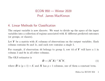
ECON 950 — Winter 2020 Prof. James MacKinnon 7. Boosting Like bagging and random forests, boosting involves creating many models. Unlike bagging and random forests, boosting creates these models sequentially, and there is no resampling involved. Boosting learns slowly by repeatedly fitting new models based on the residuals of earlier models. For regression trees, the algorithm works as follows: 1. Set ˆ f ( x ) = 0 and r i = y i for all i . 2. For m = 1 , . . . , M , repeat: i. Fit a tree ˆ f m ( x ) with d splits to the training data ( x , r ). ii. Update ˆ f by adding a shrunken version of ˆ f m ( x ) to it: f ( x ) ← ˆ ˆ f ( x ) + λ ˆ f m ( x ) . (1) Slides for ECON 950 1
iii. Update the residuals: r i ← r i − λ ˆ f m ( x i ) . (2) 3. The boosted model is M ˆ ∑ λ ˆ f m ( x ) . f ( x ) = (3) m =1 Recall that the initial value of ˆ f was 0 . Thus all of the explanatory power comes from the ˆ f m ( x ). There are three tuning parameters: 1. The number of (in this case) trees. There is a risk of overfitting if M gets too large, so we need to use cross-validation. 2. The shrinkage parameter λ . Typical values are 0.01 and 0.001. When λ is very small, M needs to be large. 3. The number of splits d , called the interaction depth . This tends to be small, perhaps just d = 1. When d = 1, every split is a stump, and (3) becomes an additive model. Slides for ECON 950 2
It seems odd that λ is not set to 1 /M . Do we have to rescale λ if M becomes larger? See ISLR Figure 8.11. For squared error loss (which may not be a good thing to use; see ESL Section 10.6), the objective function is N N ) 2 . ∑ ∑ ( ) ( L y i , f ( x i ) = y i − f ( x i ) (4) i =1 i =1 Since we build up the f ( x i ) slowly in (1), we see that y i , ˆ y i , ˆ f ( x i ) + λ ˆ f m ( x i ) ( ) ( ) L f ( x i ) ← L ) 2 y i − ˆ f ( x i ) − λ ˆ ( f m ( x i ) (5) = ) 2 , r i − λ ˆ ( f m ( x i ) = where r i is simply the i th residual for the current model, before we have added the m th term to it. Slides for ECON 950 3
At each step in the boosting algorithm, we add λ times the term ˆ f m ( x i ) that best fits the function N ) 2 , r i − ˆ ∑ f m ( x i ) ( (6) i =1 which just depends on the current residuals and on ˆ f m ( x i ). The discussion above assumes that we use a tree to obtain ˆ f m ( x i ), but many other models can also be boosted. It does not make sense to boost a linear regression model, because the residuals are orthogonal to all the predictors. 7.1. AdaBoost.M1 for two-way classification We code the output as {− 1 , 1 } instead of { 0 , 1 } . The error rate on the training sample is N err = 1 ∑ ( ) y i ̸ = G ( x i ) , (7) I N i =1 Slides for ECON 950 4
where G ( x i ) denotes the classifier. It also takes values {− 1 , 1 } . A weak classifier is only slightly better than random guessing. Boosting sequentially applies the weak classifier to repeatedly modified versions of the data (in the regression case above, these were residuals). Eventually, we have M of these, denoted G m ( x ) for m = 1 , . . . , M . We then combine these as follows to produce the final prediction ( M ) ∑ G ( x ) = sign α m G m ( x ) , (8) m =1 where the weights α m have to be determined. Instead of using residuals from successive steps, classification uses weights that change as the algorithm proceeds. Observations that were misclassified get more weight, and observations that were correctly classified get less weight. The AdaBoost.M1 algorithm works as follows: Slides for ECON 950 5
1. Initialize the observations weights to 1 /N for all i . 2. For m = 1 , . . . , M : i. Fit a classifier G m ( x ) to the training data using weights w i . ii. Compute ∑ N ( ) i =1 w i I y i ̸ = G m ( x i ) err m = . ∑ N i =1 w i ( ) iii. Compute α m = log (1 − err m ) / err m . ( ) ( ) iv. Set w i ← w i exp α m I y i ̸ = G m ( x i ) for i = 1 , . . . , N . (∑ M ) 3. The final classifier is given in (8): G ( x ) = sign m =1 α m G m ( x ) . The algorithm just described is called “Discrete AdaBoost,” because the classifier always reports − 1 or 1. A modified version called “Real AdaBoost” was proposed in Friedman, Hastie, and Tibshirani ( AMS , 2000). This seems to be a key paper. Real AdaBoost yields real numbers in the [0 , 1] interval as outputs instead of {− 1 , 1 } . Slides for ECON 950 6
In the above algorithm, step 1. is unchanged. Step 2. becomes 2. For m = 1 , . . . , M : i. Fit a classifier p m ( x ) to the training data using weights w i . ii. Compute f m = 1 ( ) 2 log p m ( x ) / (1 − p m ( x )) . ( ) iii. Set w i ← w i exp − y i f m ( x i ) for all i , and renormalize so that ∑ N i =1 w i = 1. 3. The final classifier is the sign of ∑ M m =1 f m ( x ). Observe that the f m here are the logs of odds ratios. ESL present a simulated example in which p = 10 and each input X j is N(0 , 1). The output is 1 if 10 ∑ X 2 j > χ 2 10 (0 . 5) = 9 . 34182 . (9) j =1 Thus, on average, half of the outputs will be 1 and half will be − 1. But, since we observe the realized random variables, we should be able to make predictions. Slides for ECON 950 7
There are 2000 training cases and 10,000 test ones. The weak classifier is a tree with two terminal nodes, a “stump.” The error rate of the initial classifier is 45.8%. After boosting with M = 400, it is only 5.8%. A single large tree has an error rate of 24.7%. See ESL, Figure 10.2. 7.2. Boosting and additive models Because boosting is additive — see (3) and (8) — it can be thought of as a form of basis expansion. Basis expansions take the form M ∑ f ( x ) = β m b ( x , γ m ) , (10) m =1 where the β m are expansion coefficients, and the b ( · ) are (usually) simple functions of x and the coefficient vectors γ m . Slides for ECON 950 8
For neural nets, the b ( · ) are sigmoid functions of linear combinations of x . For MARS, the b ( · ) are splines, and the γ m parametrize the variables and the values for the knots. For trees, the γ m parametrize the split variables and split points. In general, we estimate this sort of model by minimizing a loss function with respect to the β m and the γ m : N ( M ) ∑ ∑ L y i , β m b ( x , γ m ) (11) i =1 m =1 This is hard if we have to minimize with respect to all parameters at once, but it can be easy if we can minimize sequentially with respect to the parameters of one basis function at a time. The idea of forward stagewise additive modeling is to minimize (11) by adding additional basis functions without modifying previous ones. This is exactly what boosting does; see (3) and the algorithm that includes it. Slides for ECON 950 9
7.3. Other issues in boosting What does AdaBoost minimize? According to ESL, it minimizes ( ) ( ) L y, f ( x ) = exp − yf ( x ) ; (12) see Section 10.4. They show that this is equivalent to minimizing the deviance ( ) ( ) ℓ y, f ( x ) = log 1 + exp( − 2 yf ( x )) , (13) which is what a logit model would minimize, except for the factor of 2 that arises because of coding the output as {− 1 , 1 } instead of { 0 , 1 } . There is a long discussion of robust and non-robust loss functions in Section 10.6. There is a detailed discussion of boosting trees in Section 10.9. The important topic of gradient boosting is discussed in Section 10.10. There are some interesting examples in Section 10.14. Slides for ECON 950 10
Recommend
More recommend
Explore More Topics
Stay informed with curated content and fresh updates.
