ECON 950 Winter 2020 Prof. James MacKinnon 1. Introduction Machine - - PowerPoint PPT Presentation

ECON 950 — Winter 2020

• Prof. James MacKinnon
• 1. Introduction

Machine learning (ML) refers to a wide variety of methods, often computationally

• intensive. Some were invented by statisticians, others by neuroscientists, and quite

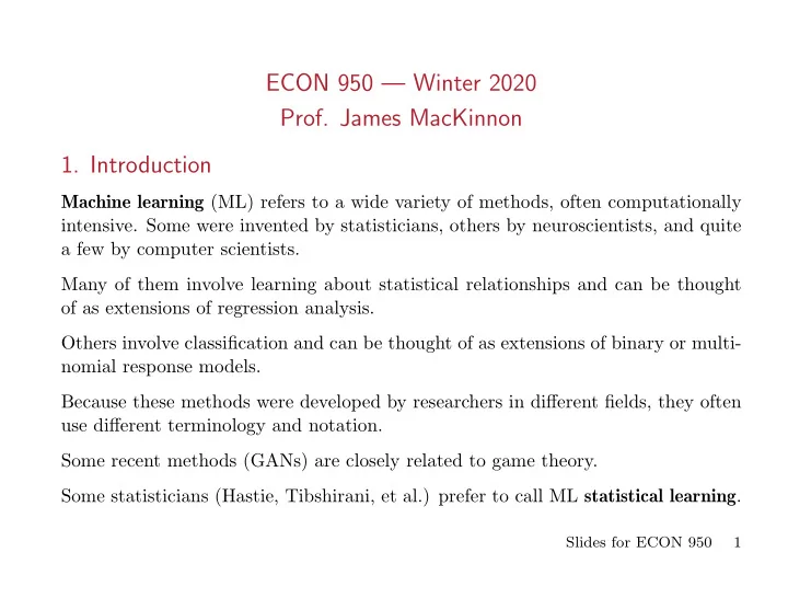
a few by computer scientists. Many of them involve learning about statistical relationships and can be thought

• f as extensions of regression analysis.

Others involve classification and can be thought of as extensions of binary or multi- nomial response models. Because these methods were developed by researchers in different fields, they often use different terminology and notation. Some recent methods (GANs) are closely related to game theory. Some statisticians (Hastie, Tibshirani, et al.) prefer to call ML statistical learning.

Slides for ECON 950 1

Principal books: Trevor Hastie, Robert Tibshirani, and Jerome Friedman, Elements of Statistical Learning, Second Edition, Springer, 2009. Gareth James, Daniela Witten, Trevor Hastie, and Robert Tibshirani, An Intro- duction to Statistical Learning, Springer, 2014. ISLR provides R code for a number of empirical examples. Trevor Hastie, Robert Tibshirani, and Martin Wainwright, Statistical Learning with Sparsity, CRC Press, 2015. Bradley Efron and Trevor Hastie, Computer Age Statistical Inference, Cambridge University Press, 2016. Ian Goodfellow, Yoshua Bengio, and Aaron Courville, Deep Learning, MIT Press, 2016. Stata 16 has added code for lasso and elastic net. Much of this code is focused on methods for inference, which is what several well-known econometricians (Belloni, Chernozhukov, Hansen, et al.) have been studying recently.

Slides for ECON 950 2

1.1. Course Requirements

• For credit, two class presentations of 20–30 minutes, or one presentation of

40–50 minutes.

• For auditors and first-year students, one presentation of 20–30 minutes.
• An essay, due at the end of July. It could be a literature review, and empirical

exercise, or a simulation study.

1.2. Course Content

• 1. Various methods for supervised learning
• 2. Model selection and cross-validation
• 3. Methods based on linear regression, including ridge regression and the lasso
• 4. Methods for classification
• 5. Kernel density estimation and kernel regression
• 6. Trees and forests

Slides for ECON 950 3

• 7. Bias, variance, and model complexity
• 8. Nonlinear models
• 9. Boosting
• 10. Numerical issues
• 11. Lasso for inference
• 12. Neural networks
• 13. Support vector machines

Both the order and the topics actually covered may differ from the above.

• 2. Supervised Learning

The objective of supervised learning is typically prediction, broadly defined. From the point of view of econometrics, it involves estimating a sort of reduced form. The learning is supervised because the data contain labeled responses. For example, picture 1 is a deer, picture 2 is a moose, picture 3 is a cow, and so on. The opposite is unsupervised learning, where data contain no labeled responses.

Slides for ECON 950 4

We might have 50,000 pictures of animals, but nothing to indicate which animals they are. Cluster analysis is an unsupervised method used for exploratory data analysis to find hidden patterns or groupings. Principal components analysis is a form of unsupervised learning that is widely used in econometrics. Generative adversarial networks, or GANs, are a recent class of machine-learning methods in which two neural networks play games with each other. A generative network generates candidate datasets, and a discriminative network evaluates them. GANs can be used to generate fake photographs that look stunningly realistic. For supervised learning, we have a training set of data, with N observations on inputs or predictors or features, together with one or more outcomes or outputs or

• responses. Often, there is just one output.

Some outputs are quantitative, often approximately continuous. The prediction task is then often called regression.

Slides for ECON 950 5

Some outputs are categorical or qualitative, in which case the prediction task is usually called classification. The distinction between regression and classification is not hard and fast. Linear regression can be used for classification. If yi is binary, we can regress it on xi to obtain fitted values xi ˆ β. Then, given a new vector x, we can classify that observation as 1 if x ˆ β ≥ 0.5 and as 0 otherwise. Of course, we do not have to use 0.5 here, and we could use a logit or probit model instead of a linear regression model. Some methods are designed for a small number of predictors, which are allowed to affect the outcomes in a very general way. Smoothing methods such as kernel regression fall into this category. Other methods are designed to handle a large number of predictors, most of which will be discarded. These are called high-dimensional methods. The best known example is the lasso. Such methods can handle problems with far more predictors than observations.

Slides for ECON 950 6

Econometricians have studied nonparametric, especially kernel, regression for a long time, although they have largely ignored other smoothing methods. Recently, econometricians have begun to study high-dimensional methods. Promi- nent names include Athey, Belloni, Chernozhukov, Hansen, and Imbens.

2.3. k-Nearest-Neighbour Methods

One simplistic approach to regression and classification is k-nearest-neighbour

• averaging. For the former, it works as follows:
• 1. For any observation with predictors x0, find the k observations with predictors

xi that are closest to x0. This could be based on Euclidean distance or on some other metric. Note that we may need to rescale some or all of the inputs so that distance is not dominated by one or a few of them. Call the set of the k closest observations Nk(x0). When k = 1, this set just contains the very closest observation, which would be x0 itself if x0 belongs to the sample.

Slides for ECON 950 7

• 2. Compute the average of the yi over all members of the set Nk(x0). Call it

ˆ y(x0). This is our prediction. kNN with k = 1 has no bias when x0 is part of the training set, but it must surely have high variance in that case. As k increases, bias goes up but variance goes down. We can use kNN for classification instead of regression. We simply classify an

• bservation with predictors x as 1 whenever ˆ

y(x) ≥ 0.5. If k = 1, this procedure always classifies every observation in the training sample correctly! There is no reason always to use 0.5. If the cost of one type of misclassification is higher than the cost of another type, we must want to use a different number. This is the first example of a bias-variance tradeoff. As k gets bigger, bias increases but variance declines.

Slides for ECON 950 8

2.4. Statistical Decision Theory

We need a loss function, of which the most common is squared error loss: L ( Y, f(X) ) = ( Y − f(X) )2. (1) Conditional on X = x, this becomes EY | X=x ( Y − f(x) )2, (2) which is minimized when f(x) equals µ(x) ≡ E(Y |X = x). (3) If we had many observations with X = x, we could simply average them, and we would get something that estimates µ(x) extremely well. But this is rarely the case. If k is large, and the k nearest neighbours are all very close to x, then we should also get something that estimates µ(x) very well. In practice, however, making k large often means that we are averaging points that are not close to x.

Slides for ECON 950 9

The larger k is, the more we are smoothing the data. Formally, we need N → ∞, k → ∞, and k/N → 0. So k has to increase more slowly than N. We can see how well a particular value of k works by using a test dataset, or holdout dataset, with M observations. The idea is to estimate the loss function by using the test dataset: MSE(k) =

M

∑

i=1

( yi − ˆ y(xi) )2, (4) where ˆ y(xi) is computed from the training set using k nearest neighbours. We can evaluate (4) for various values of k to see which one works best. Depending on how the data are actually generated, kNN may work much better or much worse than regression methods.

• kNN assumes that µ(x) is well approximated by a locally constant function.
• In contrast, linear regression assumes that µ(x) is well approximated by a

globally linear function.

Slides for ECON 950 10

• Polynomial regression assumes that µ(x) is well approximated by a globally

polynomial function.

• For samples where there are plenty of observations near the values of x that

interest us, kNN can work well.

• It may work better than polynomial regression if the function cannot be fit well

using a low-order polynomial.

• It can work well if f(x) contains both steep and flat segments, which would be

hard to approximate using a polynomial. See ISLR-fig-3.17-19.pdf.

2.5. Restricted Models

In principle, we could minimize SSR(f) =

N

∑

i=1

( yi − f(xi) )2 (5) with respect to the function f(·).

Slides for ECON 950 11

But any function that passes through all training points would fit perfectly. We have to impose restrictions on f(x). Various methods differ in how they do this. We can either limit the ways in which f(x) varies within small neighbourhoods of x, or we can limit the size of the neighbourhoods. The larger is the neighbourhood, the stronger are the constraints. The less f(x) is allowed to vary near x, or the more restrictive the ways in which it can vary, the stronger are the constraints.

2.6. Kernel Methods and Local Regression

In general, SSR(fθ, x0) =

N

∑

i=1

Kλ(x0, xi) ( yi − fθ(xi) )2, (6) where Kλ(x0, xi) is the kernel function, which depends on a parameter λ (or h),

• ften called the bandwidth, and fθ(xi) is a (usually simple) function which depends
• n a parameter vector θ.

Slides for ECON 950 12

One popular kernel function is the standard normal PDF. In that case, Kλ(x0, xi) = 1 λϕ ( ||xi − x0||/λ ) . So (6) gives more weight to points that are “close” to x0. In the univariate case, simple examples of fθ(x) include

• fθ(x) = θ0
• fθ(x) = θ0 + θ1x
• fθ(x) = θ0 + θ1x + θ2x2

For the one-dimensional case, the simplest type of kernel regression (Nadaraya- Watson) simply estimates f(x0) as ˆ f(x0) = 1 λN

N

∑

i=1

ϕ (xi − x0 λ ) yi. (7) This is just a weighted average of the yi, with more weight given to points near x0. As x0 changes, the weights change, and so ˆ f(x0) changes.

Slides for ECON 950 13

Nearest-neighbour methods are just kernel methods with a rather naive data- dependent bandwidth: Kk(xi, x0) = I ( ||xi − x0|| ≤ ||x(k) − x0|| ) , (8) where x(k) is the training observation ranked k th in distance from x0. How much weight an observation xi gets depends on how many observations are nearer to x0 than it is. The weight is 1 if there are no more than k such observations, and 0 otherwise.

2.7. Roughness Penalty and Bayesian Methods

The idea is to penalize functions that vary too much locally. In general, we have PSSR(f; λ) = SSR(f) + λJ(f), (9) where J will be large for functions that vary too rapidly within small regions of the input space.

Slides for ECON 950 14

An example is the cubic smoothing spline PSSR(f; λ) =

N

∑

i=1

( yi − f(xi) )2 + λ ∫ ( f ′′(x) )2dx. (10) The penalty here applies to the second derivative of f. For λ = 0, there is no penalty. As λ → ∞, the penalty imposed on functions that are not linear becomes prohibitive. Many types of penalty functions can be devised. For additive models, it would make sense to have f(x) =

p

∑

j=1

fj(xj) and J(f) =

p

∑

j=1

J(fj). (11) Projection pursuit regression models have f(x) =

M

∑

m=1

gm(αm

⊤x)

(12)

Slides for ECON 950 15

for adaptively chosen directions αm, and the gm functions can each have an associ- ated roughness penalty. Penalty functions are often equivalent to regularization methods, of which the best known is ridge regression. It uses ℓ2-regularization. For the linear regression model y = Xβ + u, the ridge regression estimator is ˆ βridge = (X⊤X + λI)−1X⊤y, (13) where λ is a complexity parameter. Observe that ˆ βridge is the solution to min ( (y − Xβ)⊤(y − Xβ) + λβ⊤β ) . (14) One big advantage of ridge regression and related methods is that X⊤X + λI is nonsingular, even if p > N. Penalty function methods have a Bayesian interpretation. Our prior belief is that the functions we seek to estimate exhibit a certain type of smooth behaviour. The penalty J corresponds to a log-prior, and the penalized SSR function corre- sponds to a log-posterior. Minimizing the latter corresponds to finding a posterior mode, whereas a fully Bayesian procedure would seek to find a posterior mean.

Slides for ECON 950 16

2.8. Basis Functions and Dictionary Methods

These include linear and polynomial regression functions, and also a wide variety

• f more flexible models. In general,

fθ(x) =

M

∑

m=1

θmhm(x). (15) The basis functions hm(x) are typically nonlinear and may include parameters that have to be estimated. The model is linear in the basis functions, with parameters θm to be estimated. Polynomial splines of degree K are represented by a sequence of M spline basis functions determined by M − K − 1 knots. The functions are piecewise polynomials of degree K between the knots, joined with continuity of degree K − 1 at the knots. For one-dimensional linear splines, the spline basis functions are b1(x) = 1, b2(x) = x, b3(x) = (x − t1)+, bm(x) = (x − tm)+, (16)

Slides for ECON 950 17

for m = 1, . . . , M − 2. Here tm is the mth knot, and (x − tm)+ = max(x − tm, 0). (17) A single-layer feed-forward neural network model with linear output weights can be thought of as an adaptive basis function method. This model is fθ(x) =

M

∑

m=1

βmΛ(bm + αm

⊤x),

(18) where Λ(z) denotes what is called the activation function in the NN literature. One (formerly) popular choice is the logistic function, Λ(z) = 1 1 + exp(−z) = exp(z) 1 + exp(x). (19) The hard part here is determining the directions αm and the bias terms bm. Adaptive basis function methods are also called dictionary methods, because we start with a large (perhaps infinite) set of candidate basis functions. This set is called a dictionary.

Slides for ECON 950 18

In recent years, there has been a great deal of work on deep learning, i.e., neural networks that have a great many layers and potentially millions (!) of parameters. These work extraordinarily well in certain contexts, such as identifying objects in photographs and generating fake photographs (via GANs). They are a key part of recent work on artificial intelligence. Recently, it has become popular to use the ReLu function, where ReLu stands for “rectified linear (activation) unit.” This function is just Λ(z) = max(0, z). (20) It has two advantages over the logistic function. The gradient does not vanish as z gets large, and it is extremely cheap to evaluate both Λ(x) and its gradient.

2.9. Model Selection

All of the methods we have discussed involve some kind of smoothing parameter or complexity parameter. For example:

• k for kNN regression;

Slides for ECON 950 19

• the bandwidth for kernel regression;
• the multiplier of the penalty term in penalty methods;
• the number of basis functions.

We cannot determine this parameter on the basis of the fit for the training sample, because we can always find values that make the model fit perfectly (e.g. k = 1 for kNN), or at least fit extremely well within the sample. The expected prediction error for kNN is EPEk(x0) = E ( ( y − ˆ fk(x0) )2 x = x0 ) . (21) This is equal to E ( y − µ(x0) )2 + E ( ˆ fk(x0) − fk(x0) )2 + E ( fk(x0) − µ(x0) )2, (22) where of course all expectations are conditional on x = x0. The first term in (22) is the irreducible error. Even if we knew µ(x), we would make mistakes, because the realization of y is random.

Slides for ECON 950 20

The second term in (22) is the variance of the prediction around its mean. The k subscript indicates the number of nearest neighbours. For other methods, we would index f(x0) and ˆ f(x0) differently. For kNN, the prediction is simply an average of k values of yi. Therefore, under the probably unrealistic assumption of independent and homoskedastic disturbances, the second term in (22) would reduce to σ2/k. The last term in (22) is the squared bias. For kNN it becomes (1 k

k

∑

ℓ=1

f(x(ℓ)) − µ(x0) )

2

, (23) where ℓ indexes the nearest neighbours to x0. This term can be expected to increase with k if µ(x) is reasonably smooth, because we are averaging over points that are further away from x0. In general, the third (squared bias) term declines with model complexity, and the second (variance) term increases. Note that, for kNN, the model becomes more complex as k diminishes.

Slides for ECON 950 21

Averaging over fewer neighbours is equivalent to imposing less stringent smoothness penalties or fewer restrictions. This leads to overfitting. If we graph prediction error for both the training sample and the test sample as a function of complexity, we should see that:

• The prediction error for the training sample declines monotonically as com-

plexity increases;

• The prediction error for the test sample initially declines and then increases as

complexity increases. We are evidently going to have to use some procedure that penalizes complexity in

• rder to avoid overfitting.

In principle, we could use a separate validation sample, like the test sample. This is easy do, and it is widely used with neural networks, where early stopping is used to guard against overfitting as estimation proceeds, but it wastes data. Unless data are very plentiful, it is usually better to employ cross-validation. This uses the training sample in an ingenious way for both estimation and validation.

Slides for ECON 950 22

2.10. Cross-Validation

The idea of cross-validation is to estimate the MSE of a nonparametric estimator by using the training sample for two purposes. Consider the leave-one-out estimator for a locally constant kernel regression: ˆ f−i(xi) = 1 λ(N − 1)

N

∑

j̸=i

1 λϕ (xj − xi λ ) yi. (24) This is just the kernel estimator of f(xi) using every observation except the ith. It is normally computed at the point x = xi, so as to get an estimate of f(xi) that does not depend on xi. It is very cheap to compute (24) for every xi in the sample, because the terms inside the summation are almost the same for each i. It is also inexpensive to compute leave-one-out estimates for regression models, including locally linear and locally quadratic ones, because there are formulas that tell us how the estimates change when observations are added or removed; see Section 2.6 of ETM.

Slides for ECON 950 23

For any choice of λ, we can compute the MSE using the ˆ f−i(xi) instead of the ˆ f(xi). The result is MSECV(λ) =

N

∑

i=1

( yi − ˆ f−i(xi) )2. (25) We then ask which value of λ yields the lowest MSE. If λ is too small, bias will be small but variance will be large. If it is too large, bias will be large but variance will be small. Ideally, cross-validation will allow us to find the optimal value of λ (or k in the kNN case). The special structure of both linear and kernel regression makes it inexpensive to compute leave-one-out estimates. But many other ML estimators do not have this convenient property. A much more generally useful procedure is K-fold cross-validation, where typically 5 ≤ K ≤ 10. For K-fold cross-validation, we divide the training sample into K folds (subsamples)

• f equal or roughly equal size.

Slides for ECON 950 24

Then we sequentially omit one fold at a time, applying the estimator to the other K − 1 folds. This gives us K sets of estimates. For k = 1, . . . , K, the estimates using all folds except the k th are then used to compute fitted values for observations in fold k. We use these fitted values to compute the mean squared prediction error for all

• bservations. This is then used to pick the optimal value of the tuning parameter(s).

In many cases, we just plot MSECV(λ) against the tuning parameter(s), which is just λ for kernel regression and k, or 1/k, for kNN regression.

Slides for ECON 950 25