ECON 950 Winter 2020 Prof. James MacKinnon 14. Double Machine - - PowerPoint PPT Presentation

ECON 950 — Winter 2020

• Prof. James MacKinnon
• 14. Double Machine Learning

There is a series of important papers on this topic by Chernozhukov and others. One that is recent and highly cited is

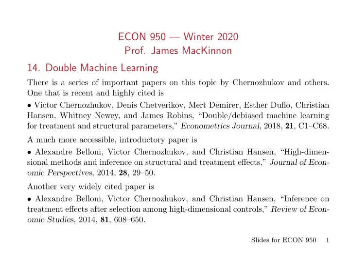
• Victor Chernozhukov, Denis Chetverikov, Mert Demirer, Esther Duflo, Christian

Hansen, Whitney Newey, and James Robins, “Double/debiased machine learning for treatment and structural parameters,” Econometrics Journal, 2018, 21, C1–C68. A much more accessible, introductory paper is

• Alexandre Belloni, Victor Chernozhukov, and Christian Hansen, “High-dimen-

sional methods and inference on structural and treatment effects,” Journal of Econ-

• mic Perspectives, 2014, 28, 29–50.

Another very widely cited paper is

• Alexandre Belloni, Victor Chernozhukov, and Christian Hansen, “Inference on

treatment effects after selection among high-dimensional controls,” Review of Econ-

• mic Studies, 2014, 81, 608–650.

Slides for ECON 950 1

An earlier paper that deals with instrumental variables is

• Alexandre Belloni, Daniel Chen, Victor Chernozhukov, and Christian Hansen,

“Sparse models and methods for optimal instruments with an application to eminent domain,” Econometrica, 2012, 80, 2369–2429.

14.1. Instrumental Variables

Using machine learning in the first stage of an IV regression is relatively easy. Consider the model y1 = γy2 + Xβ + u, E(uu⊤) = σ2I, (1) where y2 is endogenous and X is predetermined. If we can find a first-stage regres- sion y2 = g(W ) + v, (2) where X needs to lie in S(W ), then we can use generalized instrumental variables (two-stage least squares) to obtain a consistent estimate of γ.

Slides for ECON 950 2

We wrote g(W ) in (2) to indicate some sort of possibly nonlinear function. But in many cases, it makes sense to write Wπ and allow for possible nonlinearities by including powers and/or cross-products of the original instruments. Assume for the moment that X is known (a very important assumption) and has far fewer than N columns. In contrast, W potentially contains a great many instruments, perhaps more than

• N. Then it is natural to use machine-learning to estimate g(W ).

In the case where g(·) is assumed to be linear, we could use either ridge regression

• r lasso. The former was studied in Carrasco (J. Econometrics, 2012).

Carrasco actually considers several regularization methods. These include Tikhonov regularization, which is essentially ridge regression, and principal components. These methods retain all the instruments, but their coefficients are shrunk towards zero, perhaps greatly shrunk. Even though the number of principal components used is often fairly small, every instrument typically gets at least some weight, because every principal component is a linear combination of all the instruments.

Slides for ECON 950 3

However, instruments that do not contribute much to the largest principal compo- nents may get very small weights. An alternative approach is to use lasso, or some variant of it. This makes sense under some kind of sparsity assumption. Belloni et al. (2012) deals with the case in which g(W ) = Wπ. They make an “ap- proximate sparsity assumption” in which, even though the number of instruments may be very large, a small subset of them can provide a good approximation. Belloni et al. (2012) do not use ordinary lasso. Instead, they use something like adaptive lasso, where each coefficient gets a different weight in the penalty term. The penalty term can be written as λ N

p

∑

j=1

|ˆ γjπj|, (3) where the ˆ γj have to be estimated. Precisely how the ˆ γj are estimated is a bit unclear. There are two estimates. The initial one just depends on the data, and the final one depends on residuals.

Slides for ECON 950 4

The value of λ also needs to be specified. It is given as a function of other things and does not seem to involve cross-validation. Belloni et al. (2012) then suggest using a post-lasso estimator, where the estimates

• f the first-stage regression are obtained by OLS regression of y2 on the instruments

selected by lasso. This avoids the shrinkage associated with lasso. Inference about γ is straightforward, at least when the instruments are strong. They just use the usual sandwich estimator. This is true even though the lasso procedure necessarily makes mistakes. But they prove that the mistakes it makes have limited consequences, in theory. The intuition is that mistakes made by the post-lasso procedure are sufficiently small that ˆ y2 approximates the unknown g(W ) function very well. This procedure apparently works well when there are many potential instruments, but only a few strong ones. It does not work well when there are many weak instruments and no strong ones. In this case, the sparsity assumption fails. Lasso may select very few instruments,

• r even none.

Slides for ECON 950 5

Belloni at al. (2012) actually proposes several different procedures, including some that involve sample splitting and ridge regression. But they don’t seem to consider Carrasco’s approach. There is a strange empirical example, which reappears (changed in various ways) in Belloni et al. (2014). The objective is to estimate the effect on home prices of judicial decisions on “takings law.” The takings-law variable is the number of pro-plaintiff appellate judicial decisions in a given year and circuit. The idea is that, when the courts support plaintiffs, property rights are more secure, and hence real estate is worth more. This variable may be endogenous. When real estate prices are low, owners may be less likely to fight expropriation. In the Belloni et al. paper, it is reported that lasso picks just one instrument. It is the number of judicial panels with one or more members with a JD from a public university, squared. This instrument was chosen from 147 instruments. There were 183 observations.

Slides for ECON 950 6

The single instrument appears to be a strong one. Its coefficient is 0.4495 with a standard error of 0.0511. In view of this, it seems strange that no others were selected. The 2SLS estimate in Belloni et al. (2012) is 0.0631 (0.0249). There are two instru- ments, identities unreported. The estimate in Belloni et al. (2014) is 0.0648 (0.0240), with the instrument reported above. In contrast, the OLS estimate is 0.0152 (0.0132). If we are to believe these re- sults, the endogeneity of the “taking-law” regressor is so great that OLS estimate is massively biased towards zero. Interestingly, the original paper by Chen and Yeh from which the example was taken has apparently never been published.

Slides for ECON 950 7

14.2. Choosing Controls

The following analysis is mostly based on Chernozhukov et al. (2018). The key earlier paper that introduced the idea of “double selection” is Belloni et al. (2014). Suppose we want to estimate the equation y = βd + g(X) + u, (4) where d is a “treatment” or “control” variable, but not one that is assigned at random, and X is a matrix that contains p control variables. There are N observations, p may be large relative to N, and the function g(X) is unknown. It might seem that we could simply use some type of machine learning procedure to estimate g(X). When p is large and any possible nonlinearities have been taken into account by including powers and cross-products in X, it might be natural to use some variant

• f lasso.

Slides for ECON 950 8

If the treatment variable were assigned at random, this approach would be unbiased and would probably work well. But suppose instead that d = h(X) + v, (5) where h(X) is also an unknown function. In the classic case where both unknown functions are linear and X is known, there is no problem. We just regress y on d and X, and the presence of the latter ensures that we obtain consistent estimates of β. We don’t even have to estimate (5). But when we don’t know g(·), we run into the problem of regularization bias. Recall that any machine-learning estimator of g(·) has to employ some sort of regularization, which induces bias. Let ˆ g denote such an estimator. Then ˆ β = (d⊤d)−1d⊤(y − ˆ g). (6) If ˆ g were unbiased, this estimator would itself be unbiased, and it would probably work well in many cases.

Slides for ECON 950 9

Unfortunately, ˆ g is not unbiased. Even if we estimate it using a different sample (as Chernzhukov et al. recommend), that does not eliminate the bias. They find that n1/2(ˆ β − β0) = (n−1d⊤d)−1n−1/2d⊤u + (n−1d⊤d)−1n−1/2d⊤(g0 − ˆ g). (7) The first term has mean 0 and is evidently Op(n−1/2). So if it were the only term, n1/2(ˆ β − β0) would have standard asymptotic properties. But the second term does not converge. The quantity n−1/2d⊤(g0 − ˆ g) is a sum of n terms, divided by n1/2. Each of these terms has a non-zero mean. Although the bias diminishes as n increases, it always does so more slowly than n−1/2. Therefore, the second term actually diverges. This does not imply that ˆ β −β0 diverges. It does not. But it converges more slowly than it should under standard asymptotics, and the bias can be large. How fast ˆ β converges to β0 depends on how fast ˆ g converges to g0. For all machine- learning methods, this is slower than n−1/2.

Slides for ECON 950 10

There are two ways to overcome this regularization bias. The key to both of them is to estimate two equations via machine learning. This is called double machine

• learning. In the lasso case (which came first), it is called double selection.

The first equation is (4), as before. The second equation is (5), the equation that explains the treatment variable. It is generally estimated in exactly the same way as (4). The idea is to “partial out” the effects of X on d. What we need to obtain are the residuals ˆ v. This leads to the estimator ˇ β = (ˆ v⊤d)−1ˆ v⊤(y − ˆ g), (8) which looks like an IV estimator. Chernozhkov et al. (2018) proves that ˇ β has good properties. They show that n1/2(ˇ β − β0) is the sum of three terms. The first term is E(v2)−1n−1/2v⊤u

d

− → N(0, Σ), (9)

Slides for ECON 950 11

where Σ is the asymptotic variance of n1/2(ˇ β − β0), which can be estimated con- sistently in the usual way. The second term is E(v2)−1n−1/2(ˆ h − h0)(ˆ g − g0). (10) This depends on the product of the estimation errors in the two equations. Even if both ˆ h and ˆ g suffer from considerable regularization bias, the product in (10) should vanish much faster than either of their squares would vanish. There is a third term as well. It will go away even without sample splitting, but sample splitting (to be discussed below) makes it go away faster. Figure 1 in Chernozhkov et al. (2018) compares the conventional and double-ML estimators for a particular simulation with n = 500 and p = 20. They use a random forest to estimate g(x) and h(X). The conventional estimator is severely biased and more spread out than asymptotic theory predicts. The double-ML estimator is slightly biased and seems to have the correct variance.

Slides for ECON 950 12

14.3. Double Selection and Partialing Out

Consider the special case of (4) in which y = βd + Xγ + u (11) and the special case of (5) in which d = Xδ + v. (12) Suppose further that X is not high-dimensional. We could simply estimate β by regressing y on d and X. Using the FWL theorem, we find that ˆ β = (d⊤MXd)−1d⊤MXy (13) But since ˆ v = MXd, ˆ β is equal to (ˆ v⊤MXd)−1ˆ v⊤MXy = (ˆ v⊤ˆ v)−1ˆ v⊤ˆ u, (14) where ˆ u is the vector of residuals from regressing y on X.

Slides for ECON 950 13

The first expression in (14) is just a special case of (8). The second one looks like the estimate from an FWL regression. The idea of double selection is to use lasso (or some other procedure) twice, once to select the regressors that belong in (4), and then to select the regressors that belong in (5). Let ˜ X denote the union of those two sets of regressors. Then run the OLS regression y = βd + ˜ Xγ + u. (15) This yields the double selection estimator ˆ β = (d⊤M ˜

Xd)−1d⊤M ˜ Xy,

(16) which looks very much like (13). The key feature of double selection is that all regressors which help to explain either d or y (according to lasso) are included as controls in (15). The FWL theorem suggests another way to proceed.

Slides for ECON 950 14

• 1. Run some sort of machine learning procedure for d on X. This could be lasso,

but it could be many other things. Stata apparently uses lasso followed by a post-lasso regression. Obtain residuals ˜ v.

• 2. Run another machine-learning procedure for y on X. Obtain residuals ˜

u.

• 3. Regress ˜

u on ˜ v. This is called partialing out. In this case, it is not essential that the two machine- learning procedures be the same. Of course, if X were low-dimensional, we could just use OLS in steps 1 and 2. The estimate from 3 would then be the right-most expression in (14). When asymptotic theory provides a good guide, one would expect the double- selection and partialing-out estimators to be similar. In the special case of (11), they would be identical.

Slides for ECON 950 15

14.4. Sample Splitting

Perhaps the biggest contribution of Chernozhukov et al. (2018) is to propose cross- fitting, which is based on sample splitting. They break the sample into K folds, each of size n = N/K. Assume for simplicity that N/k is an integer. Denote the k th fold by Ik and its complement by Ic

k.

They construct a machine-learning estimator ˇ βk for each fold, using the observations in Ic

k to estimate the tuning parameter(s).

Chernozhukov et al. (2018) suggest that K = 4 and K = 5 work better than K = 2. In its implementation of a special case, Stata defaults to K = 10. In the simplest approach (DML1), they average the estimators ˇ βk across the K folds to obtain ˜ β. There is another variant called DML2, in which they solve an optimization problem to obtain ˜ β rather than simply averaging the ˇ βk. In certain cases, DML2 is actually easy, and it is the default for Stata.

Slides for ECON 950 16

Consider the partialing-out estimator (14). It is just the estimate of β from a simple regression of ˆ u on ˆ v. For DML2, instead of taking ˆ u and ˆ v from post-lasso regressions over the entire sample, we form each of them from K subvectors, one for each of the folds. In case this is not enough work, Chernozhukov et al. recommend repeating the entire procedure S times, where each involves a different random split into K folds. They recommend using the median of the ˜ βs as the reported estimate. They also recommend reporting a particular estimate of the variance of the median. Much of the theory is in a very general framework. In later parts of the paper, they go back and look at the partially linear model (4) and (5). They also look at a related model where the regressor of interest is endogenous. There are three empirical examples. They use various machine-learning methods: lasso (but what version?), a single regression tree, random forest, boosted regression trees, a particular neural network, and two methods that combine other methods. There are some interesting regularities across all three examples:

Slides for ECON 950 17

• The choice of machine-learning method does not substantively change any con-
• clusions. This accords with the theory.
• Using the median method to account for uncertainty due to sample splitting in-

creases standard errors relative to just using conventional methods that simply condition on ˆ v and ˆ u. Stata 16 implements several procedures based on cross-fit partialing out. They all use lasso and are based on DML2. By default, K = 10. They do not seem to repeat the procedure S times and compute the median.

Slides for ECON 950 18