ECON 950 Winter 2020 Prof. James MacKinnon 11. Neural Networks - PowerPoint PPT Presentation
ECON 950 Winter 2020 Prof. James MacKinnon 11. Neural Networks Neural networks go back many decades, but they have recently become a very hot topic because of major improvements in performance. ESL says that the most widely used neural
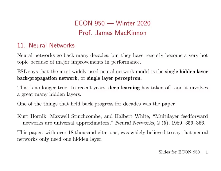
ECON 950 — Winter 2020 Prof. James MacKinnon 11. Neural Networks Neural networks go back many decades, but they have recently become a very hot topic because of major improvements in performance. ESL says that the most widely used neural network model is the single hidden layer back-propagation network , or single layer perceptron . This is no longer true. In recent years, deep learning has taken off, and it involves a great many hidden layers. One of the things that held back progress for decades was the paper Kurt Hornik, Maxwell Stinchcombe, and Halbert White, “Multilayer feedforward networks are universal approximators,” Neural Networks , 2 (5), 1989, 359–366. This paper, with over 18 thousand citations, was widely believed to say that neural networks only need one hidden layer. Slides for ECON 950 1
Abstract: This paper rigorously establishes that standard multilayer feedforward networks with as few as one hidden layer using arbitrary squashing functions are capable of approximating any Borel measurable function from one finite dimensional space to another to any desired degree of accuracy, provided sufficiently many hidden units are available. In this sense, multilayer feedforward networks are a class of universal approximators. For regression, there is typically one output Y at the top of the network diagram. For classification, there are typically K of them, denoted Y k . At the bottom are p inputs. In between are M activation functions which explain derived features Z m , K target functions that map from the Z m to T k , and K output functions g k ( T ) which map from the T k to the Y k . The activation functions for the derived features are Z m = σ ( α 0 m + x ⊤ α m ) , (1) Slides for ECON 950 2
where the choice of σ ( · ) has changed over time. For many years, the most popular choice for the activation function was the sigmoid function , which we call the logistic function: 1 exp( x ) σ ( x ) = 1 + exp( − x ) = 1 + exp( x ) . (2) The target function that aggregates the Z m is T k = β 0 k + zβ k (3) The output function is typically the identity for a regression, so that g k ( T ) = T k . For classification, it is more common to use the softmax function exp( T k ) g k ( T ) = , (4) ∑ K ℓ =1 exp( T ℓ ) which is just the transformation used for multinomial logit. Slides for ECON 950 3
Combining the activation functions with the output function, we obtain fitted values f k ( x ) = g k ( T ) via (1), (3), and (4). Because we do not observe the Z m , the units that compute them are called hidden units . There can be more than one layer of these. If we think of the Z m as basis expansions of the original inputs, a neural network is like a linear or multilogit model that uses them as inputs. But, unlike basis expansions, parameters of the activation functions are estimated. For any sigmoid function, we can scale and/or recenter the input. Evidently, σ ( x/ 2) rises more slowly than σ ( x ), and σ (2 x ) rises faster. If we change the function from σ ( x ) to σ ( x − x 0 ), we shift the threshold where σ > 0 . 5 from 0 to x 0 . If || α || is very small, the sigmoid function will be almost linear. If || α || is very large, the sigmoid function will be very flat near 0, then very steep, then very flat near 1. Slides for ECON 950 4
The neural network model with one hidden layer has the same form as the projection pursuit regression model. The difference is that the activation functions have a particular functional form. Recall that the PPR can be written as M ∑ g m ( x ⊤ ω m ) , y = (5) m =1 Suppose that g m ( x ⊤ ω m ) = β m σ ( α 0 m + x ⊤ α m ) (6) = β m σ ( α 0 m + || α m || x ⊤ ω m ) , where ω = α m / || α m || is a unit vector. Evidently (6) is a very special case of the ridge function g m ( x ⊤ ω m ). Because the activation functions in neural nets are much more restrictive than ridge functions in PPR, we tend to need a lot more of them. Slides for ECON 950 5
For some years, the hyperbolic tangent or tanh function was popular as the activa- tion function. Recall that tanh( x ) = e 2 x − 1 e 2 x + 1 . (7) While the logistic function ranges from 0 to 1, tanh( x ) ranges from − 1 to 1. Both the logistic and tanh functions seem natural, because they map smoothly from the real line to an interval. However, they turned out to have important deficiencies. • They both “saturate”. When the argument is small, the logistic will be close to 0, and when the argument is large, it will be close to 1. • Changing the weights (the α m vectors) has little effect when the functions are saturated. • This is closely related to the “vanishing gradient problem.” When the activa- tion function is saturated, the gradients are very small, so it is hard to know how to vary the weights. These problems tend to be especially severe for models with several layers. If saturation occurs for any layer, making changes to the weights for lower layers will have little impact on the model fit. Slides for ECON 950 6
In econometric terms, identification becomes extremely difficult. The solution is to use the rectified linear activation unit , or ReLU as the activation function. This function is simply g ( x ) = max(0 , x ) , (8) which is absurdly easy to calculate. It saturates if the argument is negative, but not if it is positive. In the latter case, the gradient never vanishes. The ReLU now seems to be the default activation function for most types of neural networks. However, there can be problems when x < 0. Therefore, it is generally good to start with positive inputs. The ReLU can also be generalized in various ways. For example, the leaky ReLU is g ( x ) = I ( x > 0) x + 0 . 01 I ( x ≤ 0) x. (9) So instead of being 0 when x is negative, it is a small negative number that has a small gradient. Slides for ECON 950 7
There are many other generalizations, including the exponential linear unit : g ( x ) = I ( x > 0) x + a I ( x ≤ 0)( e x − 1) . (10) where a is a hyperparameter to be tuned. 11.1. Fitting Neural Networks Neural networks generally have a lot of unknown parameters, often called weights . The complete set is the vector θ . It consists of α 0 m and α m , m = 1 , . . . , M [ M ( p + 1)] (11) for the activation functions, plus β 0 k and β k , k = 1 , . . . , K [ K ( M + 1)] (12) for the target functions. Slides for ECON 950 8
For regression, the objective function is N K N ) 2 . ∑ ∑ ∑ ( R ( θ ) = R i ( θ ) = y ik − f k ( x i ) (13) i =1 k =1 i =1 Here, following ESL, we allow there to be more than one output, although it seems odd that there is no allowance for these to be correlated. For classification, a sensible objective function is the deviance: N K N ∑ ∑ ∑ R ( θ ) = R i ( θ ) = y ik log f k ( x i ) . (14) i =1 k =1 i =1 The corresponding classifier for any x is the value of k that maximizes f k ( x ). With the softmax activation function (4), minimizing (14) is equivalent to estimat- ing a linear logistic regression in the hidden units. If we simply minimize (13) or (14), we are likely to overfit, perhaps severely. Slides for ECON 950 9
The obvious solution is to regularize, but that does not seem to be what neural net folks do, perhaps because there are too many parameters. Instead, they stop the algorithm early, before actually getting to the minimum. This involves using a validation sample as estimation progresses. However, this means that starting values are important. With ReLU, it would be really bad to start at a point where a lot of the activation functions equal 0. Minimizing R ( θ ) can be done by back-propagation , which is a two-pass procedure. Starting values are often chosen randomly. Back-propagation often works well, especially on parallel computers, because each hidden unit passes information only to and from units with which it is connected. However, back-propagation can be slow, and better methods are available. For the regression case, K ) 2 . ∑ ( R i ( θ ) = y ik − f k ( x i ) (15) k =1 Slides for ECON 950 10
The derivatives with respect to the β km are ∂R i ( ) g ′ ⊤ β k ) z mi , = − 2 y ik − f k ( x i ) k ( z i (16) ∂β km ⊤ α m ), and z i is an M -vector with typical element z mi . where z mi = σ ( α 0 + x i The derivatives with respect to the α mℓ are K ∂R i ∑ g ′ ⊤ β k ) β km σ ′ ( x i ⊤ α m ) x iℓ . ( ) = − 2 y ik − f k ( x i ) k ( z i (17) ∂α mℓ k =1 A gradient descent update at iteration j + 1 has the form N ∂R i β ( j +1) = β ( j ) ∑ km − γ j km ∂β ( j ) i =1 km , (18) N ∂R i α ( j +1) = α ( j ) ∑ mℓ − γ j mℓ ∂α ( j ) i =1 mℓ Slides for ECON 950 11
where γ j is the learning rate . We can rewrite the derivatives in (16) and (17) as ∂R i = δ ki z mi (19) ∂β km and ∂R i = s mi x iℓ . (20) ∂α mℓ For example, ( ) g ′ ⊤ β k ) , δ ki = − 2 y ik − f k ( x i ) k ( z i (21) and we can see from (17) that s mi is even more complicated. We can think of δ ki and s mi as “errors” from the current model at the output and hidden layer unit, respectively. These errors satisfy the back-propagation equations K ∑ s mi = σ ′ ( x i ⊤ α m ) β km δ ki . (22) k =1 Slides for ECON 950 12
Recommend
More recommend
Explore More Topics
Stay informed with curated content and fresh updates.
