ECON 950 Winter 2020 Prof. James MacKinnon 4. Linear Methods for - PowerPoint PPT Presentation
ECON 950 Winter 2020 Prof. James MacKinnon 4. Linear Methods for Classification The output variable is now discrete. We want to divide up the space of the input variables into a collection of regions associated with K different predicted
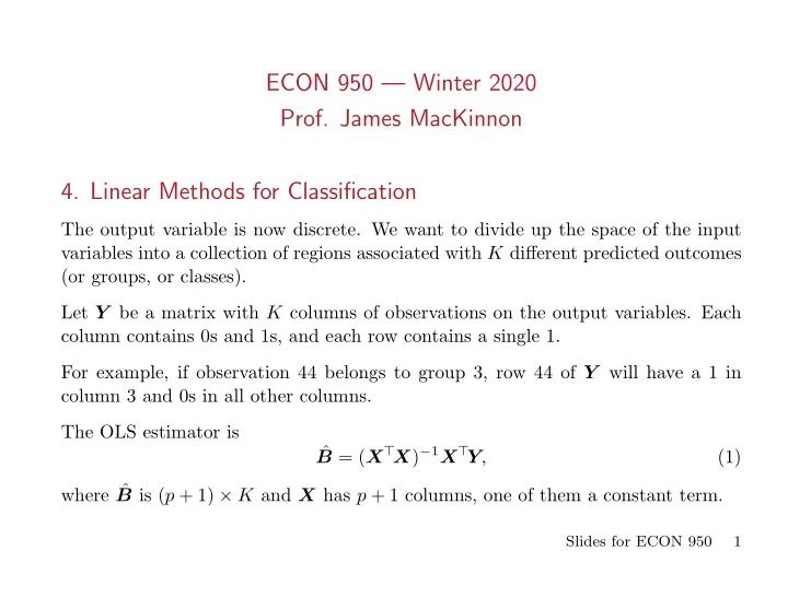
ECON 950 — Winter 2020 Prof. James MacKinnon 4. Linear Methods for Classification The output variable is now discrete. We want to divide up the space of the input variables into a collection of regions associated with K different predicted outcomes (or groups, or classes). Let Y be a matrix with K columns of observations on the output variables. Each column contains 0s and 1s, and each row contains a single 1. For example, if observation 44 belongs to group 3, row 44 of Y will have a 1 in column 3 and 0s in all other columns. The OLS estimator is ˆ B = ( X ⊤ X ) − 1 X ⊤ Y , (1) where ˆ B is ( p + 1) × K and X has p + 1 columns, one of them a constant term. Slides for ECON 950 1
This is a generalization of the linear probability model . The latter is used when there are only two outcomes. In that case, we can use just one regression, because the fitted values must sum to 1 over all the equations. In general, we could get away with estimating K − 1 regressions and obtaining the fitted values for the K th by using this property. For any input vector x , we can calculate the fitted output ˆ f ( x ) = [1 , x ⊤ ] ˆ B , which is a K -vector. Then we classify x as belonging to group (or class, or region) k if k corresponds to the largest element of ˆ f ( x ). Unfortunately, as ESL explains, linear regression often performs very badly when K ≥ 3. The problem is “masking,” where middle classes get missed. ESL works through an example where the largest value of x ⊤ ˆ B k is always for one of the two extreme classes, even though it is easy to see visually that there are three classes which can be separated without error. This example is shown in ESL-fig4.02.pdf. Slides for ECON 950 2
4.1. Linear Discriminant Analysis Suppose that f k ( x ) is the density of X in class k , where k runs from 1 to K . Suppose that π k is the prior probability of class k , where the event G = k means that the class actually is k . Then, by Bayes’ theorem, π k f k ( x ) Pr( G = k | x ) = . (2) ∑ K ℓ =1 π ℓ f ℓ ( x ) So we just need to find the f k ( x ) and combine them with the prior probabilities. If the density of each class is multivariate normal, ( ) 1 − 1 2 ( x − µ k ) ⊤ Σ − 1 − f k ( x ) = (2 π ) p/ 2 | Σ k | 1 / 2 exp k ( x − µ k ) . (3) In the case of linear discriminant analysis , we assume that Σ k = Σ for all k . Slides for ECON 950 3
In general, the log of the ratio of the posteriors (that is, the log odds) is log π k + log f k ( x ) f ℓ ( x ) . (4) π ℓ When the densities are given by (3) with constant Σ , this reduces to log π k − 1 2 ( x − µ k ) ⊤ Σ − 1 ( x − µ k ) + 1 2 ( x − µ ℓ ) ⊤ Σ − 1 ( x − µ ℓ ) . − − (5) π ℓ Because the two covariance matrices are the same, this simplifies to log π k − 1 2 ( µ k − µ ℓ ) ⊤ Σ − 1 ( µ k − µ ℓ ) + x ⊤ Σ − 1 ( µ k − µ ℓ ) , − (6) π ℓ which is linear in x . Since this is true for any pair of classes, all boundaries must be hyperplanes. Where else have we seen a model in which the log of the odds is linear in x ? The logistic regression or logit model! Slides for ECON 950 4
The linear discriminant function for class k is δ k ( x ) = x ⊤ Σ − 1 µ k − 1 ⊤ Σ − 1 µ k + log π k . − (7) 2 µ k We simply classify x as belonging to the class k for which (7) is largest. Of course, for all the classes, we need to estimate π k = N k /N, ˆ (8) ∑ µ k = 1 ˆ (9) x i N k i ∈ G k K ∑ ∑ 1 ˆ µ k ) ⊤ ( x i − ˆ µ k )( x i − ˆ Σ = . (10) N − K k =1 i ∈ G k Here G k is the set of observations that belong to class k . Since the values of δ k ( x ) depend on the ˆ π k , we could change the boundaries of the classes by using different estimates of the π k . Slides for ECON 950 5
For example, we could shrink them towards 1 /K : π k ( α ) = αN k N + (1 − α ) 1 ˆ K . (11) When N is small and the N k are not too different, this ought to produce better results by accepting more bias in return for less variance. ESL discusses the relationship between LDA and classification by linear regression. For two classes, there is a close relationship. 4.2. Quadratic Discriminant Analysis If the Σ k matrices are not equal, then the log odds does not simplify to (6). In contrast to (7), the discriminant functions are now quadratic in x . The quadratic discriminant functions are δ k ( x ) = − 1 2 log | Σ k | − 1 2 ( x − µ k ) ⊤ Σ − 1 − − k ( x − µ k ) + log π k . (12) Slides for ECON 950 6
Now we have to estimate separate covariance matrices for each class: ∑ Σ k = 1 ˆ µ k ) ⊤ ( x i − ˆ µ k )( x i − ˆ . (13) N k i ∈ G k Note that these matrices are p × p , each with p ( p + 1) / 2 parameters to estimate. Especially when some of the N k are small, the Σ k may not be estimated very well, which will probably cause the classification procedure to perform much worse on the test data than on the training data. There is an interesting alternative to QDA that is based on LDA. Simply augment x by adding all squares and cross-products, and then perform LDA. See ESL-fig4.01.pdf and ESL-fig4.06.pdf. Of course, this also adds a lot of parameters if p is large. ESL reports that LDA and QDA often work remarkably well, even though the Gaussian assumption, and the equal covariance matrix assumption, are surely not true in the vast majority of cases. Slides for ECON 950 7
Presumably, the parsimony of LDA causes it to have low variance but high bias. In many cases, it is apparently worth accepting a lot of bias in return for low variance. Perhaps the data can only support simple decision boundaries such as linear or quadratic ones, and the estimates provided via the Gaussian LDA and QDA models are stable. Since we need | ˆ Σ k | and ˆ rather than just ˆ Σ − 1 Σ , it is convenient to use the eigen k decomposition ˆ ⊤ . Σ k = U k D k U k (14) Then p ∑ log | ˆ Σ k | = log d kℓ , (15) ℓ =1 and ( ) ( ) µ k ) ⊤ ˆ Σ − 1 ⊤ D − 1 ⊤ ( x − ˆ ⊤ ( x − ˆ ( x − ˆ k ( x − ˆ µ k ) = U k µ k ) U k µ k ) . (16) k Getting the eigenvalues and eigenvectors is expensive, but it gives us the determi- nant and the inverse almost for free. Slides for ECON 950 8
4.3. Regularized Discriminant Analysis We can shrink the covariance matrices towards their average: Σ k ( α ) = α ˆ ˆ Σ k + (1 − α ) ˆ Σ . (17) Of course, α has to be chosen, perhaps by cross-validation. Similarly, we could shrink ˆ σ 2 I : Σ towards the scalar covariance matrix ˆ Σ ( γ ) = γ ˆ ˆ σ 2 I . Σ + (1 − γ )ˆ (18) Combining (17) and (18), we could use ( ) Σ k ( α, γ ) = α ˆ ˆ γ ˆ σ 2 I Σ k + (1 − α ) Σ + (1 − γ )ˆ , (19) which has two tuning parameters to specify. In Section 4.3.3, ESL goes on to discuss reduced-rank LDA, which is closely related to LIML and to Johansen’s approach to cointegration. Slides for ECON 950 9
4.4. Logistic Regression The log of the odds between any two classes is assumed to be linear in x . This implies that exp( β k 0 + x ⊤ β k ) Pr( G = k | x ) = p k ( x , θ ) = , (20) 1 + ∑ K − 1 ℓ =1 exp( β ℓ 0 + x ⊤ β ℓ ) where θ contains all of the parameters. There are ( K − 1) ∗ ( p + 1) of these. ESL discusses ML estimation of the logit model ( K = 2) in Section 4.4.1. What they have there, and later in Section 4.4.3 on inference, is closely related to the material in Sections 11.2 and 11.3 of ETM. They do not discuss estimation of the multinomial logit (multilogit) model except in Exercise 4.4. For binary logit, the probability of class 1 is ⊤ β ) exp( β 0 + x i 1 p ( x , θ ) = ⊤ β ) = ⊤ β ) . (21) 1 + exp( β 0 + x i 1 + exp( − β 0 − x i Slides for ECON 950 10
Thus the contributions to the loglikelihood are ( ) ⊤ β − log ⊤ β ) β 0 + x i 1 + exp( β 0 + x i if y i = 1 (22) and ( ) ⊤ β ) − log 1 + exp( β 0 + x i if y i = 0 . (23) The sum of these contributions over all observations is the loglikelihood function: ( ) N ∑ ( ) ⊤ β ) − log ⊤ β ) ℓ ( β ) = y i ( β 0 + x i 1 + exp( β 0 + x i . (24) i =1 To maximize ℓ ( β ), we differentiate with respect to β 0 and each element of β and set the derivatives to 0. The first-order condition for β 0 is interesting: N N ∑ ∑ ⊤ β ) exp( β 0 + x i y i − ⊤ β ) = 0 . (25) 1 + exp( β 0 + x i i =1 i =1 Slides for ECON 950 11
So the sum of the y i must be equal to the sum of the probabilities that y = 1. Thus, at the ML estimates, the expected number of 1s must equal the actual number. This is similar to the condition for OLS that the mean of the regressand must equal the mean of the fitted values. The loglikelihood (24) can be maximized by a quasi-Newton method that is equiv- alent to iteratively reweighted least squares. See ESL, p. 121 or ETM pp. 455-456. 4.5. Regularized Logistic Regression Of course, we can penalize the loglikelihood function for (multinomial) logit, using either an L 1 or L 2 penalty, or perhaps both in the fashion of the elastic-net penalty. ESL only discusses the L 1 (lasso) case. For the logit/lasso case, instead of maximizing ( )) N ∑ ( ⊤ β ) − log ⊤ β ) y i ( β 0 + x i 1 + exp( β 0 + x i , (26) i =1 Slides for ECON 950 12
Recommend
More recommend
Explore More Topics
Stay informed with curated content and fresh updates.
