FMS161/MASM18 Financial Statistics Lecture 2, Linear Time Series - PowerPoint PPT Presentation
FMS161/MASM18 Financial Statistics Lecture 2, Linear Time Series Erik Lindstrm Systems with discrete time Linear systems space models form while being causal time-invariant stationary Discrete time models are written as a difference
FMS161/MASM18 Financial Statistics Lecture 2, Linear Time Series Erik Lindström
Systems with discrete time Linear systems space models form while being causal time-invariant stationary Discrete time models are written as a difference equation Impulse Response - h s t or h Transfer Function - H z Frequency Function - H e i 2 f Typical process: The SARIMAX-process ◮ Can be represented on a polynomial or state ◮ Stability ◮ Lyapunov stable, ∥ x ( t ) − x e ∥ < ϵ ◮ Asympt. stable lim t →∞ ∥ x ( t ) − x e ∥ = 0
Systems with discrete time Linear systems space models form while being Discrete time models are written as a difference equation Impulse Response - h s t or h Transfer Function - H z Frequency Function - H e i 2 f Typical process: The SARIMAX-process ◮ Can be represented on a polynomial or state ◮ Stability ◮ Lyapunov stable, ∥ x ( t ) − x e ∥ < ϵ ◮ Asympt. stable lim t →∞ ∥ x ( t ) − x e ∥ = 0 ◮ causal ◮ time-invariant ◮ stationary
Systems with discrete time Linear systems space models form while being equation Typical process: The SARIMAX-process ◮ Can be represented on a polynomial or state ◮ Stability ◮ Lyapunov stable, ∥ x ( t ) − x e ∥ < ϵ ◮ Asympt. stable lim t →∞ ∥ x ( t ) − x e ∥ = 0 ◮ causal ◮ time-invariant ◮ stationary ◮ Discrete time models are written as a difference ◮ Impulse Response - h ( s , t ) or h ( τ ) ◮ Transfer Function - H ( z ) ◮ Frequency Function - H ( e i 2 π f )
Systems with discrete time Linear systems space models form while being equation Typical process: The SARIMAX-process ◮ Can be represented on a polynomial or state ◮ Stability ◮ Lyapunov stable, ∥ x ( t ) − x e ∥ < ϵ ◮ Asympt. stable lim t →∞ ∥ x ( t ) − x e ∥ = 0 ◮ causal ◮ time-invariant ◮ stationary ◮ Discrete time models are written as a difference ◮ Impulse Response - h ( s , t ) or h ( τ ) ◮ Transfer Function - H ( z ) ◮ Frequency Function - H ( e i 2 π f )
Impulse response non-Gaussian) has a well defined impulse we let the input be 1 at time zero and then zero for the rest of the time. It is the convolution of the input u and the impulse response h . ◮ A causal linear stable system (Gaussian or response h ( · ) . ◮ The impulse response is the output of a system if ◮ The output for a general input u is given as ∞ ∑ y ( t ) = h ( i ) u ( t − i ) = ( h ∗ u )( t ) i = 0
Difference equations interpretation of the operations) structure: Transfer Function (which can be defined also for a system not following this linear difference equation) (1) Difference equation representation for ARX/ARMA 0 with (the latter equation with a Z-transform y t + a 1 y t − 1 + · · · + a p y t − p = u t + b 1 u t − 1 + · · · + b q u t − q using the delay operator, zy t = y t − 1 leads to the y t = 1 + b 1 z 1 + · · · + b q z q 1 + a 1 z 1 + · · · + a p z p u t = B ( z ) A ( z ) u t = H ( z ) u t ∞ ∑ h ( τ ) z − τ ; H ( z ) = Y ( Z ) = H ( Z ) U ( Z )
Frequency representation The frequency function is defined from the transfer function as H giving a amplitude and phase shift of an input trigonometric signal, as e.g. ( e i 2 π f ) = H ( f ) u ( k ) = cos ( 2 π fk ) y ( k ) = |H ( f ) | cos ( 2 π fk + arg ( H ( f ))) | f | ≤ 0 . 5
Spectrum The spectrum at frequency f is the average Note: The covariance is not symmetric for (2) energy in the output with frequency f . multivariate processes (think Granger causality) spectrum of i.i.d. zero mean random variables with variance one, through a linear system with ◮ If we filter standard white noise, i.e. a sequence frequency function H then we get a signal with R ( f ) = |H ( f ) | 2 . ◮ The spectrum is also the Fourier transform of covariance function γ ( k ) = E [ X n X n − k ] with ∞ ∞ γ ( k ) e − i 2 π fk [ γ ( · ) is sym ] ∑ ∑ R ( f ) = = γ ( k ) cos ( 2 π fk ) . k = −∞ k = −∞
Inverse filtering in discrete time AIM: Reconstruct the input u from the output y signal. linear, stable, and time-invariant. It then follows that (3) k , or equivalently that there exists causal and stable g such that NOTE: The causality means that we do reconstruct ◮ Assume that we have a filter g with ( h ) being w ( k ) = ( g ∗ y )( k ) = ( g ∗ h ∗ u )( k ) ◮ We say that g is an inverse if w ( k ) = u ( k ) for all ∃ ( g ∗ h )( k ) = δ ( k ) G ( z ) H ( z ) = 1 the signal from old values, h ( k ) = 0 ∀ k < 0.
ARMA(p,q)-filter ◮ The process is defined as y t + a 1 y t − 1 + · · · + a p y t − p = x t + c 1 x t − 1 + · · · + c q x t − q ◮ The corresponding transfer function is given by H ( z ) = 1 + c 1 z 1 + · · · + c q z q 1 + a 1 z 1 + · · · + a p z p = C ( z ) A ( z ) ◮ Properties: ◮ Frequency Function as H ( e i 2 π f ) , f ∈ ( − 0 . 5 , 0 . 5 ] ◮ Stability: Poles to A ( z − 1 ) = 0, st | π i | < 1 , i = 1 , . . . , p ◮ Invertability: Zeroes to C ( z − 1 ) = 0, st | η i | < 1 , i = 1 , . . . , q
ARMAX process We can combine moving average (MA) and exogenous variables in the ARMAX process (4) Or in transfer function form y t + a 1 y t − 1 + · · · + a p y t − p = x t + b 1 x t − 1 + · · · + b q x t − q + e t + c 1 e t − 1 + · · · + c r e t − r y t = B ( z ) A ( z ) x t + C ( z ) A ( z ) e t
Auto correlation and cross-correlation (5) and corresponding autocorrelation function (6) (7) and corresponding autocorrelation function (8) ◮ The auto covariance is defined as γ ( k ) = E [ Y t Y t + k ] ρ ( k ) = γ ( k ) γ ( 0 ) ◮ The cross covariance is defined as γ XY ( k ) = E [ X t Y t + k ] ρ XY ( k ) = γ XY ( k ) γ XY ( 0 )
Auto covariance for ARMA (9) (10) This is known as the Yule-Walker equation. ◮ Consider the ARMA(p,q) process Y t + a 1 Y t − 1 + . . . a p Y t − p = e t + . . . c q e t − q ◮ The auto covariance then satisfies γ ( k )+ a 1 γ ( k − 1 )+ . . . a p γ ( k − p ) = c k γ eY ( 0 )+ . . . c q γ eY ( q − k ) ◮ Proof: Multiply with Y t − k , and use that E [ e t − l Y t − k ] = 0 for k > l
Cointegration non-standard. ◮ It is rather common that financial time series { X ( t ) } are non-stationary, often integrated ◮ This means that ∇ X ( t ) is typically stationary. We then say that is an integrated process, X ( t ) ∼ I ( 1 ) . ◮ Assume that the processes X ( t ) ∼ I ( 1 ) and Y ( t ) ∼ I ( 1 ) but X ( t ) − β Y ( t ) ∼ I ( 0 ) . We then say that X ( t ) and Y ( t ) are cointegrated . ◮ NOTE: that the asymptotic theory for β is
Log-real money and Bond rates 1974-1985 Figure: Log-real money and interest rates Levels Differences 12.1 0.1 12 11.9 Money 0.05 11.8 11.7 0 11.6 11.5 −0.05 1975 1980 1985 1975 1980 1985 Levels Differences 0.22 0.01 0.2 0 0.18 Bond rate 0.16 −0.01 0.14 −0.02 0.12 −0.03 0.1 −0.04 1975 1980 1985 1975 1980 1985
Estimation Two dominant approaches PEM, GMM) We focus on the optimization based estimators today. ◮ Optimization based estimation (LS, WLS, ML, ◮ Matching properties (MM, GMM, EF, ML, IV)
General properties Implications... p Where ◮ Denote the true parameter θ 0 ◮ Introduce an estimator ˆ θ = T ( X 1 , . . . , X N ) ◮ Observation: The estimator is a function of data. ◮ Bias: b = ( E [ T ( X )] − θ 0 ) . ◮ Consistency: T ( X ) → θ 0 . ◮ Efficiency: Var ( T ( X )) ≥ I N ( θ 0 ) − 1 . [ ] ∂ 2 I N ( θ 0 ) ij = − E ℓ ( X 1 , . . . , X N , θ ) , ∂θ i ∂θ j | θ = θ 0 [ ∂ ℓ ( X 1 , . . . , X N , θ ) ∂ ] = C ov ℓ ( X 1 , . . . , X N , θ ) T ∂θ i ∂θ j | θ = θ 0 where ℓ is the log-likelihood function.
Estimators (11) (12) F The maximum likelihood estimator is defined as N The asymptotics for the MLE is given by Hint: MLmax will help you during the labs and project. N ˆ ∑ θ MLE = arg max ℓ ( θ ) = arg max log p θ ( x n | x 1 , . . . x n − 1 ) n = 1 √ ( ) d ( ) ˆ 0 , I − 1 θ MLE − θ 0 → N .
Estimators N (15) with (14) The general so-called M estimator (ex GMM) is (16) The asymptotics for that estimator is given by (13) defined as ˆ θ = arg min Q ( θ ) = arg min log Q ( θ ) √ ( ) d ( 0 , J − 1 IJ − 1 ) ˆ θ − θ 0 → N . J = E [ ∇ θ ∇ θ log Q ] I = E [( ∇ θ log Q ) ( ∇ θ log Q ) T ]
ML methods for Gaussian processes vector of parameters. (17) (18) If we can calculate the likelihood, then it follows that we can use a standard optimization routine ◮ Say that we have sample Y = { y t } , t = 1 , 2 , , . . . , n from a Gaussian process. We then have that Y ∈ N ( µ ( θ ) , Σ( θ )) , where θ is a ◮ The log-likelihood for Y can be written as ℓ ( Y , θ ) = − 1 2 log ( det ( 2 π Σ( θ ))) 2 ( Y − µ ( θ )) T Σ( θ ) − 1 ( Y − µ ( θ )) . − 1 to maximize ℓ ( Y , θ ) and thereby estimate θ .
Example: AR(2) x 2 . . . . . x 1 . x N . x 3 . . Solve! Explanation on blackboard Y = , X = x N − 1 x N − 2 Then ˆ θ = ( X T X ) − 1 ( X T Y ) . ( ∑ x 2 ∑ x i − 1 x i − 2 ) i − 1 ( X T X ) = ∑ x i − 1 x i − 2 ∑ x 2 i − 2 ( ∑ x i x i − 1 ) and ( X T Y ) = ∑ x i x i − 2
Recommend
More recommend
Explore More Topics
Stay informed with curated content and fresh updates.

