ECON 950 Winter 2020 Prof. James MacKinnon 5. Kernel Density - PowerPoint PPT Presentation
ECON 950 Winter 2020 Prof. James MacKinnon 5. Kernel Density Estimation Two useful books are Li and Racine (2007) and Henderson and Parmeter (2015). The simplest way to estimate a CDF graphically is to use the empirical distribution function
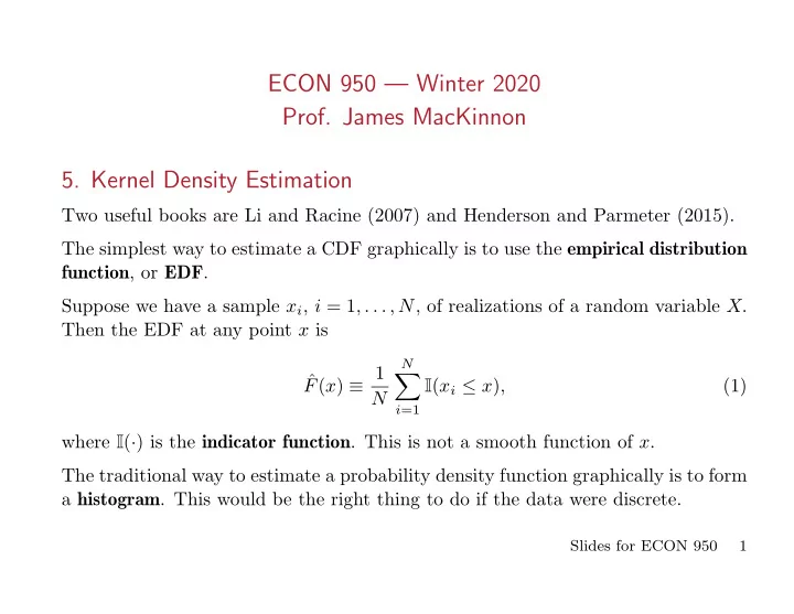
ECON 950 — Winter 2020 Prof. James MacKinnon 5. Kernel Density Estimation Two useful books are Li and Racine (2007) and Henderson and Parmeter (2015). The simplest way to estimate a CDF graphically is to use the empirical distribution function , or EDF . Suppose we have a sample x i , i = 1 , . . . , N , of realizations of a random variable X . Then the EDF at any point x is N ∑ F ( x ) ≡ 1 ˆ I ( x i ≤ x ) , (1) N i =1 where I ( · ) is the indicator function . This is not a smooth function of x . The traditional way to estimate a probability density function graphically is to form a histogram . This would be the right thing to do if the data were discrete. Slides for ECON 950 1
The interval containing the x i is partitioned into a set of subintervals by a set of points z j , j = 1 , . . . , M , with z j < z j +1 for all j , where typically M < < N . Like the EDF, the histogram is a locally constant function with discontinuities. Unlike the EDF, the histogram is discontinuous at the z j , not the x i . Let j be such that z j ≤ x < z j +1 for some x . Then the histogram is just the following estimate of the density function at x : N ∑ f ( x ) = 1 I ( z j ≤ x i < z j +1 ) ˆ . (2) N z j +1 − z j i =1 The value of the histogram at x is the proportion of the sample points contained in the same bin as x , divided by the length of the bin. A histogram is extremely dependent on the choice of the partitioning points z j . With just two z j , the histogram would look like a uniform distribution with lower limit z 1 and upper limit z 2 . With a great many z j , many bins would be empty. The remaining bins would contain spikes, because z j +1 − z j would tend to 0 as the partition became finer. Slides for ECON 950 2
We want neither too few nor too many bins. To prove anything about asymptotic validity, we would need a rule for increasing the number of bins as N → ∞ . 5.1. Kernel estimation of distribution functions The discontinuous indicator function I ( x i ≤ x ) in (1) can be interpreted as the CDF of a degenerate random variable which puts all its probability mass on x i . The EDF can be thought of as the unweighted average of these CDFs. We can obtain a smooth estimator of the CDF by replacing the discontinuous func- tion I ( x ≥ x i ) in (1) by a continuous CDF that has support in an interval contain- ing x i . This will give us a weighted average. Let K ( z ) be any continuous CDF corresponding to a distribution with mean 0. This function is called a cumulative kernel . It usually corresponds to a distribution with a density that is symmetric around the origin, such as the standard normal. In order to be able to control the degree of smoothness of the estimate, we set the variance of the distribution characterized by K ( z ) to 1 and introduce the bandwidth parameter h as a scaling parameter. Slides for ECON 950 3
This gives the kernel CDF estimator ( x i − x ) N ∑ F h ( x ) = 1 ˆ K . (3) N h i =1 This estimator depends on the cumulative kernel K ( · ) and the bandwidth h . As h → 0, a typical term of the summation on the right-hand side of (3) tends to I ( x i ≥ x ) = I ( x ≤ x i ), and so ˆ F h ( x ) tends to the EDF ˆ F ( x ) as h → 0. At the other extreme, as h becomes large, a typical term of the summation tends to the constant value K (0), which makes ˆ F h ( x ) very much too smooth. In the usual case in which K ( z ) corresponds to a symmetric distribution, ˆ F h ( x ) tends to 0 . 5 as h → ∞ . It has been shown that h = 1 . 587 sN − 1 / 3 is optimal for CDF estimation, where s is the standard deviation of the x i . Here “optimal” means that we minimize the asymptotic mean integrated squared error , or AMISE ; see below. Slides for ECON 950 4
5.2. Kernel estimation of density functions For density estimation, we can choose K ( z ) to be not only continuous but also differentiable. Then we define the kernel function , often simply called the kernel , as k ( z ) ≡ K ′ ( z ). If we differentiate equation (3) with respect to x , we obtain the kernel density estimator ( x i − x ) N ∑ 1 ˆ f h ( x ) = k . (4) Nh h i =1 Notice that we divide by Nh rather than just N . Like the kernel CDF estimator (3), the kernel density estimator (4) depends on the choice of kernel k ( · ) and the bandwidth h . One very popular choice for k ( · ) is the Gaussian kernel , which is just the standard normal density ϕ ( · ). It gives a positive (although perhaps very small) weight to every point in the sample. Slides for ECON 950 5
Another commonly used kernel, which has certain optimality properties, is the Epanechnikov kernel , √ k 1 ( z ) = 3(1 − z 2 / 5) √ for | z | < 5 , 0 otherwise . (5) 4 5 √ This kernel gives a positive weight only to points for which | ( x i − x ) | /h < 5. Yet another popular kernel is the biweight kernel : k 2 ( z ) = 15 16(1 − z 2 ) 2 I ( | z | ≤ 1) . (6) This is quite similar to the Epanechnikov kernel, but it squares the argument and involves different constants. Three properties shared by all these kernels, and other second-order kernels , are ∫ ∞ κ 0 ( k ) ≡ k ( z ) dz = 1 , (7) −∞ ∫ ∞ κ 1 ( k ) ≡ zk ( z ) dz = 0 , (8) −∞ Slides for ECON 950 6
and ∫ ∞ z 2 k ( z ) dz < ∞ . κ 2 ( k ) ≡ (9) −∞ The first property is shared by all PDFs. The second property is that the kernel has first moment zero. It is satisfied by any kernel that is symmetric about zero. The third property is that the kernel has finite variance. It is essential for estimates based on the kernel k to have finite bias. The big difference between the Epanechnikov and Gaussian kernels is that the √ former is 0 for | z | > 5, while the latter is always positive. It can be shown that, to highest order, the bias of the kernel estimator is ( ˆ ) ∼ = h 2 2 f ′′ ( x ) κ 2 ( k ) , E f h ( x ) − f ( x ) (10) where f ′′ ( x ) is the second derivative of the density f ( x ). Recall from (9) that κ 2 ( k ) is the second moment of the kernel k . Slides for ECON 950 7
Notice that the bias does not depend directly on the sample size. It only depends on N through h , which should become smaller as N increases. Since bias is proportional to h 2 , it may seem that we should make h very small. But that turns out to be desirable only when N is very large. The shape of the density matters. If the slope of the density is constant, then f ′′ ( x ) = 0, and there is no bias. It can also be shown that, to highest order, the variance of ˆ f h ( x ) is ( ˆ ) 2 ∼ 1 E f h ( x ) − f ( x ) Nhf ( x ) R ( k ) , (11) = where ∫ k 2 ( z ) dz R ( k ) = (12) measures the “difficulty” of the kernel. Note that the variance depends inversely on both the sample size and the bandwidth. Slides for ECON 950 8
It makes sense that the variance goes up as h goes down, because fewer observations are averaged to give us the estimate for any x . In choosing h , there is a tradeoff between bias and variance. A larger h increases bias but reduces variance. Making h larger is like making k larger in k NN estimation. The asymptotic mean squared error , or AMSE , is ( ˆ ) = Bias 2 ( ˆ ) ( ˆ ) AMSE f h ( x ) f h ( x ) + Var f h ( x ) (13) ( ) 2 h 4 + ( Nh ) − 1 f ( x ) R ( k ) . ∼ = 1 4 κ 2 f ′′ ( x ) − 2 ( k ) If we held h fixed as N → ∞ , the first term (bias squared) would stay constant, and the second term (variance) would go to zero. Thus we want to make h smaller as N increases. But we need to ensure that Nh → ∞ as N → ∞ to make the second term go away. The AMSE depends on x , so it will be different in different parts of the distribution. Slides for ECON 950 9
There is no law requiring h to be the same for all x , although using more than one value risks causing visible artifacts where h changes. If our objective is simply to draw a picture that looks nice and accurately portrays the true distribution, we may well want to use more than one value of h , but we will have to smooth out the artifacts. To get an overall result, it is common to consider the asymptotic mean integrated squared error , or AMISE : ∫ ∞ ( ˆ ) ( ˆ ) AMISE f h ( x ) = AMSE f h ( z ) dz −∞ (14) 2 ( k ) R ( f ′′ ) + R ( k ) = 1 ∼ 4 h 4 κ 2 − nh , where R ( f ′′ ) measures the “roughness” of f ( x ). Note that R ( f ′′ ) should not be confused with R ( k )! Larger values of R ( f ′′ ) imply that the density is harder to estimate. AMISE involves the same tradeoff between bias and variance as AMSE, but it does not depend on x because we have integrated it out. Slides for ECON 950 10
The Epanechnikov kernel is optimal, in the sense that it minimizes AMISE. The efficiency of some other kernel, say k g ( · ), relative to k 1 ( · ) is R ( k g ) κ 2 ( k g ) 1 / 2 . (15) R ( k 1 ) The quantity κ 2 ( k 1 ) does not appear here, because κ 2 ( k 1 ) = 1. The loss in efficiency relative to Epanechnikov is roughly 0.61% for biweight and 5.13% for Gaussian. 5.3. Bandwidth selection The choice of bandwidth is far more important than the choice of kernel. The optimal bandwidth for minimizing AMSE is ( ) 1 / 5 f ( x ) R ( k ) h opt = N − 1 / 5 . (16) ( ) 2 κ 2 2 ( k ) f ′′ ( x ) and the optimal bandwidth for minimizing AMISE is ( ) 1 / 5 R ( k ) h opt = N − 1 / 5 . (17) κ 2 2 ( k ) R ( f ′′ ) Slides for ECON 950 11
Recommend
More recommend
Explore More Topics
Stay informed with curated content and fresh updates.
