Single Factor Experiments: Estimating the Parameters In the means - - PowerPoint PPT Presentation

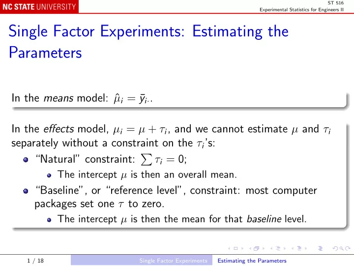
ST 516 Experimental Statistics for Engineers II

Single Factor Experiments: Estimating the Parameters

In the means model: ˆ µi = ¯ yi·. In the effects model, µi = µ + τi, and we cannot estimate µ and τi separately without a constraint on the τi’s: “Natural” constraint: τi = 0;

The intercept µ is then an overall mean.

“Baseline”, or “reference level”, constraint: most computer packages set one τ to zero.

The intercept µ is then the mean for that baseline level.

1 / 18 Single Factor Experiments Estimating the Parameters

ST 516 Experimental Statistics for Engineers II

R command for “effects” model

summary(lm(EtchRate ~ factor(Power), data = etchRateLong))

Output

Call: lm(formula = EtchRate ~ factor(Power), data = etchRateLong) Residuals: Min 1Q Median 3Q Max

• 25.4
• 13.0

2.8 13.2 25.6 Coefficients: Estimate Std. Error t value Pr(>|t|) (Intercept) 551.200 8.169 67.471 < 2e-16 *** factor(Power)180 36.200 11.553 3.133 0.00642 ** factor(Power)200 74.200 11.553 6.422 8.44e-06 *** factor(Power)220 155.800 11.553 13.485 3.73e-10 ***

• Signif. codes:

0 *** 0.001 ** 0.01 * 0.05 . 0.1 1 Residual standard error: 18.27 on 16 degrees of freedom Multiple R-Squared: 0.9261, Adjusted R-squared: 0.9122 F-statistic: 66.8 on 3 and 16 DF, p-value: 2.883e-09

2 / 18 Single Factor Experiments Estimating the Parameters

ST 516 Experimental Statistics for Engineers II

R command for “means” model

# to get the means model, suppress the intercept in the formula: summary(lm(EtchRate ~ 0 + factor(Power), etchRateLong))

Output

Call: lm(formula = EtchRate ~ 0 + factor(Power), data = etchRateLong) Residuals: Min 1Q Median 3Q Max

• 25.4
• 13.0

2.8 13.2 25.6 Coefficients: Estimate Std. Error t value Pr(>|t|) factor(Power)160 551.200 8.169 67.47 <2e-16 *** factor(Power)180 587.400 8.169 71.90 <2e-16 *** factor(Power)200 625.400 8.169 76.55 <2e-16 *** factor(Power)220 707.000 8.169 86.54 <2e-16 ***

• Signif. codes:

0 *** 0.001 ** 0.01 * 0.05 . 0.1 1

3 / 18 Single Factor Experiments Estimating the Parameters

ST 516 Experimental Statistics for Engineers II

Graphical Comparison of Means (Not recommended) Montgomery suggests a graphical presentation of the mean response by factor:

curve(dt((x - 552.2)/8.169, df = 16)/8.169, from = 530, to = 730) abline(v = 552.2, lty = 2) curve(dt((x - 587.4)/8.169, df = 16)/8.169, add = TRUE) abline(v = 587.4, lty = 2) curve(dt((x - 625.4)/8.169, df = 16)/8.169, add = TRUE) abline(v = 625.4, lty = 2) curve(dt((x - 707.0)/8.169, df = 16)/8.169, add = TRUE) abline(v = 707.0, lty = 2)

Can you visualize sliding one curve to a position where all the means could be sampled from that distribution? If so, the population means might be equal. If not, they most likely are not equal.

4 / 18 Single Factor Experiments Estimating the Parameters

ST 516 Experimental Statistics for Engineers II

Interval Estimates

One-at-a-time 100(1 − α)% confidence intervals: For a treatment mean µi: ¯ yi· ± tα/2,N−a

• MSE

n . For a pairwise difference µi − µj: ¯ yi· − ¯ yj· ± tα/2,N−a

• 2MSE

n .

5 / 18 Single Factor Experiments Estimating the Parameters

ST 516 Experimental Statistics for Engineers II

Fisher’s Least Significant Difference Note that for a single pair of means µi and µj, we reject H0 : µi = µj if and only if |¯ yi· − ¯ yj·| > tα/2,N−a

• 2MSE

n . The right hand side is Fisher’s Least Significant Difference, or LSD. R command

library("agricolae") print(LSD.test(lm(EtchRate ~ factor(Power), data = etchRateLong), "factor(Power)"))

6 / 18 Single Factor Experiments Estimating the Parameters

ST 516 Experimental Statistics for Engineers II

Output

$statistics Mean CV MSerror LSD 617.75 2.957095 333.7 24.49202 $parameters Df ntr t.value 16 4 2.119905 $means EtchRate std r LCL UCL Min Max 160 551.2 20.01749 5 533.8815 568.5185 530 575 180 587.4 16.74216 5 570.0815 604.7185 565 610 200 625.4 20.52559 5 608.0815 642.7185 600 651 220 707.0 15.24795 5 689.6815 724.3185 685 725 $groups trt means M 1 220 707.0 a 2 200 625.4 b 3 180 587.4 c 4 160 551.2 d

7 / 18 Single Factor Experiments Estimating the Parameters

ST 516 Experimental Statistics for Engineers II

A Problem: Multiplicity Each interval is an assertion: “µi − µj lies between two values”. The probability that the assertion is wrong is α (often 5%). If we make many such assertions, we should expect around 5% of them to be wrong. If we make all pairwise comparisons among a treatments, we make a(a − 1)/2 assertions. E.g. for a = 7 that’s 21 assertions, so we expect roughly one to be wrong.

8 / 18 Single Factor Experiments Estimating the Parameters

ST 516 Experimental Statistics for Engineers II

A Solution: Simultaneous Confidence Intervals The probability that any of a collection of confidence intervals is wrong is the experiment-wise error rate. The probability that one specified confidence interval is wrong is the comparison-wise error rate. Sometimes we use confidence intervals with a given comparison-wise error rate, like those on an earlier slide. Sometimes, e.g. when we need to rank the treatments, we need to control the experiment-wise error rate. Methods: Bonferroni, Scheff´ e, Tukey, Dunnett.

9 / 18 Single Factor Experiments Estimating the Parameters

ST 516 Experimental Statistics for Engineers II

The key to controlling the experiment-wise error rate is to make the intervals wider, to reduce the error rate. The Bonferroni approach for N intervals is to construct each of them with comparison-wise rate α/N; the experiment-wise error rate is then at most α. The Tukey approach uses the “Honestly Significant Difference” or HSD, and gives an experiment-wise error rate exactly α.

10 / 18 Single Factor Experiments Estimating the Parameters

ST 516 Experimental Statistics for Engineers II

R command

TukeyHSD(aov(EtchRate ~ factor(Power), data = etchRateLong))

Output

Tukey multiple comparisons of means 95% family-wise confidence level Fit: aov(formula = EtchRate ~ factor(Power), data = etchRateLong) $‘factor(Power)‘ diff lwr upr p adj 180-160 36.2 3.145624 69.25438 0.0294279 200-160 74.2 41.145624 107.25438 0.0000455 220-160 155.8 122.745624 188.85438 0.0000000 200-180 38.0 4.945624 71.05438 0.0215995 220-180 119.6 86.545624 152.65438 0.0000001 220-200 81.6 48.545624 114.65438 0.0000146

11 / 18 Single Factor Experiments Estimating the Parameters

ST 516 Experimental Statistics for Engineers II

Balance; Unbalanced Designs

A design with the same number n of runs for each level of the factor is balanced. Sometimes we may have different sample sizes: ni runs for level i. By chance: e.g. one or more measurements has to be excluded from the analysis because of incorrect procedures. By design: if we are interested in making comparisons between

• ne distinguished level, the control level, and each of the others,

we may use more runs at the control level, to gain precision. Formulas for F0 and CIs change to reflect lack of balance.

12 / 18 Single Factor Experiments Estimating the Parameters

ST 516 Experimental Statistics for Engineers II

Model Adequacy Checking

Using the F-distribution to assess F0 and using the t-distribution to set up CIs both depend on the data being normally distributed with constant variance. Checks are based on residuals ei,j = yi,j − ˆ yi,j where in the single-factor model ˆ yi,j = ˆ µi = ¯ yi·.

13 / 18 Single Factor Experiments Estimating the Parameters

ST 516 Experimental Statistics for Engineers II

Probability plot (quantile-quantile plot) of pooled residuals: may reveal outliers, other departures from normality. Time plot (residuals in time order): may reveal correlation. Residuals versus fitted values: may reveal non-constant variance; e.g. variance changes systematically with mean. logarithms, but also square roots, other powers (Box-Cox).

14 / 18 Single Factor Experiments Estimating the Parameters

ST 516 Experimental Statistics for Engineers II

In R, use the residuals() and fitted() methods on the object returned by either the lm() or aov() function. E.g. for the etch-rate data:

etchRateLm <- lm(EtchRate ~ factor(Power), data = etchRateLong) # quantile-quantile plot of pooled residuals: qqnorm(residuals(etchRateLm), datax = TRUE) # plot residuals versus fitted values: plot(fitted(etchRateLm), residuals(etchRateLm)) # to better see non-constant variance, plot abs(residuals): plot(fitted(etchRateLm), abs(residuals(etchRateLm)))

You can also plot the object itself: plot(etchRateLm) produces a standard set of graphs.

15 / 18 Single Factor Experiments Estimating the Parameters

ST 516 Experimental Statistics for Engineers II

A data set that suggests transformation: peak discharge rate, estimated using 4 methods (peak-discharge.txt).

peakDischarge <- read.table("data/peak-discharge.txt", header = TRUE) peakDischargeLong <- reshape(peakDischarge, varying = 2:7, v.names = "Discharge", timevar = "Obs", idvar = "Code", direction = "long") boxplot(Discharge ~ Method, peakDischargeLong) boxplot(sqrt(Discharge) ~ Method, peakDischargeLong)

16 / 18 Single Factor Experiments Estimating the Parameters

ST 516 Experimental Statistics for Engineers II

• 1

2 3 4 5 10 15

Peak discharge rates

17 / 18 Single Factor Experiments Estimating the Parameters

ST 516 Experimental Statistics for Engineers II

• 1

2 3 4 1 2 3 4

Peak discharge rates (sqrt scale)

18 / 18 Single Factor Experiments Estimating the Parameters