Two-Factor Design: Estimating Model Parameters Recall the model: y i - PowerPoint PPT Presentation
ST 516 Experimental Statistics for Engineers II Two-Factor Design: Estimating Model Parameters Recall the model: y i , j , k = + i + j + ( ) i , j + i , j , k For balanced data, with the natural constraints: E ( y ) =
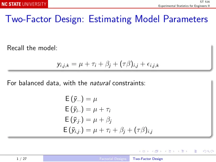
ST 516 Experimental Statistics for Engineers II Two-Factor Design: Estimating Model Parameters Recall the model: y i , j , k = µ + τ i + β j + ( τβ ) i , j + ǫ i , j , k For balanced data, with the natural constraints: E (¯ y ··· ) = µ E (¯ y i ·· ) = µ + τ i E (¯ y · j · ) = µ + β j E (¯ y i , j · ) = µ + τ i + β j + ( τβ ) i , j 1 / 27 Factorial Designs Two-Factor Design
ST 516 Experimental Statistics for Engineers II So the natural parameter estimates are µ = ¯ ˆ y ··· τ i = ¯ ˆ y i ·· − ˆ µ = ¯ y i ·· − ¯ y ··· ˆ β j = ¯ y · j · − ˆ µ = ¯ y · j · − ¯ y ··· � � � τ i + ˆ ( τβ ) i , j = ¯ y i , j · − µ + ˆ ˆ β j = ¯ y i , j · − ¯ y i ·· − ¯ y · j · + ¯ y ··· These are also least squares estimates. 2 / 27 Factorial Designs Two-Factor Design
ST 516 Experimental Statistics for Engineers II Standard packages use the “reference level” constraints. E.g., the battery life data R commands # for more compact output: batteryLife$M <- factor(batteryLife$Material) batteryLife$T <- factor(batteryLife$Temperature) summary(lm(Life ~ M * T, batteryLife)) Output Call: lm(formula = Life ~ M * T, data = batteryLife) Residuals: Min 1Q Median 3Q Max -60.750 -14.625 1.375 17.938 45.250 3 / 27 Factorial Designs Two-Factor Design
ST 516 Experimental Statistics for Engineers II Output, continued Coefficients: Estimate Std. Error t value Pr(>|t|) (Intercept) 134.75 12.99 10.371 6.46e-11 *** M2 21.00 18.37 1.143 0.263107 M3 9.25 18.37 0.503 0.618747 T70 -77.50 18.37 -4.218 0.000248 *** T125 -77.25 18.37 -4.204 0.000257 *** M2:T70 41.50 25.98 1.597 0.121886 M3:T70 79.25 25.98 3.050 0.005083 ** M2:T125 -29.00 25.98 -1.116 0.274242 M3:T125 18.75 25.98 0.722 0.476759 --- Signif. codes: 0 *** 0.001 ** 0.01 * 0.05 . 0.1 1 Residual standard error: 25.98 on 27 degrees of freedom Multiple R-squared: 0.7652, Adjusted R-squared: 0.6956 F-statistic: 11 on 8 and 27 DF, p-value: 9.426e-07 4 / 27 Factorial Designs Two-Factor Design
ST 516 Experimental Statistics for Engineers II R note For convenience, you can get the same output using: with(batteryLife, {M <- factor(Material); T <- factor(Temperature); summary(lm(Life ~ M * T))}) But this way does not add the variables M and T to batteryLife . If you use within() instead of with() , the new variables are added: batteryLife <- within(batteryLife, {M <- factor(Material); T <- factor(Temperature)}) summary(lm(Life ~ M * T, batteryLife)) 5 / 27 Factorial Designs Two-Factor Design
ST 516 Experimental Statistics for Engineers II Additive Model: No Interactions Model is y i , j , k = µ + τ i + β j + ǫ i , j , k Use with care–first test significance of interactions; In ANOVA table without interactions , “Error” line results from pooling Df and SS for “Interactions” and “Error” from the table with interactions. With balanced data, main effect sums of squares and mean squares do not change, but F -ratios and P -values generally do change. 6 / 27 Factorial Designs Two-Factor Design
ST 516 Experimental Statistics for Engineers II Example: Battery life # Interaction model summary(aov(Life ~ M * T, batteryLife)) Df Sum Sq Mean Sq F value Pr(>F) M 2 10684 5341.9 7.9114 0.001976 ** T 2 39119 19559.4 28.9677 1.909e-07 *** M:T 4 9614 2403.4 3.5595 0.018611 * Residuals 27 18231 675.2 --- Signif. codes: 0 *** 0.001 ** 0.01 * 0.05 . 0.1 1 # Additive model summary(aov(Life ~ M + T, batteryLife)) Df Sum Sq Mean Sq F value Pr(>F) M 2 10684 5341.9 5.9472 0.006515 ** T 2 39119 19559.4 21.7759 1.239e-06 *** Residuals 31 27845 898.2 --- Signif. codes: 0 *** 0.001 ** 0.01 * 0.05 . 0.1 1 7 / 27 Factorial Designs Two-Factor Design
ST 516 Experimental Statistics for Engineers II One Observation per Cell Only a single replicate: y i , j = µ + τ i + β j + ( τβ ) i , j + ǫ i , j Degrees of freedom for error = ab ( n − 1) = 0, so we cannot test the usual hypotheses about main effects and interactions. Additive (no-interaction) model may still be fitted, and we can test for a less general form of interactions. 8 / 27 Factorial Designs Two-Factor Design
ST 516 Experimental Statistics for Engineers II Tukey’s One Degree of Freedom for Non-Additivity Assumes structured interactions ( τβ ) i , j = γτ i β j . Can fit with one observation per cell, and test H 0 : γ = 0. Sum of squares is �� a � �� 2 � b SS A + SS B + y 2 j =1 y i , j y i · y · j − y ·· ·· i =1 ab SS N = ab SS A SS B Break this out as a separate line in the ANOVA table. Tukey’s ODOFNA is not implemented in some packages; ANOVA table can be found by including squared fitted values in model, after the other effects. 9 / 27 Factorial Designs Two-Factor Design
ST 516 Experimental Statistics for Engineers II Example: impurity data impurity.txt; the ANOVA line for I(fitted(a)^2) is the same as that for “Nonadditivity” in Example 5.2: impurity <- read.table("data/impurity.txt", header = TRUE) a <- aov(Impurity ~ factor(Temperature) + factor(Pressure), impurity) summary(a) Df Sum Sq Mean Sq F value Pr(>F) factor(Temperature) 2 23.333 11.667 46.667 3.885e-05 *** factor(Pressure) 4 11.600 2.900 11.600 0.002063 ** Residuals 8 2.000 0.250 summary(aov(Impurity ~ factor(Temperature) + factor(Pressure) + I(fitted(a)^2), impurity)) Df Sum Sq Mean Sq F value Pr(>F) factor(Temperature) 2 23.3333 11.6667 42.9491 0.0001174 *** factor(Pressure) 4 11.6000 2.9000 10.6759 0.0042006 ** I(fitted(a)^2) 1 0.0985 0.0985 0.3627 0.5660026 Residuals 7 1.9015 0.2716 10 / 27 Factorial Designs Two-Factor Design
ST 516 Experimental Statistics for Engineers II General Factorial Design More than two factors. Terms in model: main effects A , B , C , . . . ; two-factor interactions AB , AC , . . . ; three-factor interactions ABC , . . . ; and so on. 11 / 27 Factorial Designs General Factorial Design
ST 516 Experimental Statistics for Engineers II E.g. three factor statistical model: y i , j , k , l = µ + τ i + β j + γ k +( τβ ) i , j +( τγ ) i , k +( βγ ) j , k +( τβγ ) i , j , k + ǫ i , j , k , l Example: Soft drink bottling (soft-drink-bottling.txt), Carbonation Pressure Speed Height 10 25 200 -3 10 25 200 -1 10 25 250 -1 10 25 250 0 10 30 200 -1 10 30 200 0 10 30 250 1 10 30 250 1 12 25 200 0 12 25 200 1 12 25 250 2 ... ... ... ... 12 / 27 Factorial Designs General Factorial Design
ST 516 Experimental Statistics for Engineers II R commands softDrinkBottling <- read.table("data/soft-drink-bottling.txt", header = TRUE) softDrinkBottling <- within(softDrinkBottling, {C <- factor(Carbonation); P <- factor(Pressure); S <- factor(Speed)}) summary(aov(Height ~ C * P * S, softDrinkBottling)) Output Df Sum Sq Mean Sq F value Pr(>F) C 2 252.750 126.375 178.4118 1.186e-09 *** P 1 45.375 45.375 64.0588 3.742e-06 *** S 1 22.042 22.042 31.1176 0.0001202 *** C:P 2 5.250 2.625 3.7059 0.0558081 . C:S 2 0.583 0.292 0.4118 0.6714939 P:S 1 1.042 1.042 1.4706 0.2485867 C:P:S 2 1.083 0.542 0.7647 0.4868711 Residuals 12 8.500 0.708 --- Signif. codes: 0 *** 0.001 ** 0.01 * 0.05 . 0.1 1 13 / 27 Factorial Designs General Factorial Design
ST 516 Experimental Statistics for Engineers II Interaction plot with(softDrinkBottling, interaction.plot(Carbonation, Pressure, Height)) Pressure 8 30 25 mean of Height 6 4 2 0 10 12 14 Carbonation 14 / 27 Factorial Designs General Factorial Design
ST 516 Experimental Statistics for Engineers II Response Curves When one or more factors is quantitative , a regression model can help in understanding the relationship. Example: battery life Temperature is quantitative; fit quadratic equations, separately by material: l <- lm(Life ~ M * (Temperature + I(Temperature^2)), batteryLife) summary(l) 15 / 27 Factorial Designs Response Curves and Surfaces
ST 516 Experimental Statistics for Engineers II Call: lm(formula = Life ~ M * (Temperature + I(Temperature^2)), data = batteryLife) Residuals: Min 1Q Median 3Q Max -60.750 -14.625 1.375 17.938 45.250 Coefficients: Estimate Std. Error t value Pr(>|t|) (Intercept) 169.380165 20.567656 8.235 7.66e-09 *** M2 -9.756198 29.087058 -0.335 0.73991 M3 -36.617769 29.087058 -1.259 0.21884 Temperature -2.501446 0.755148 -3.313 0.00264 ** I(Temperature^2) 0.012851 0.005260 2.443 0.02139 * M2:Temperature 2.328099 1.067941 2.180 0.03815 * M3:Temperature 3.404339 1.067941 3.188 0.00361 ** M2:I(Temperature^2) -0.018512 0.007439 -2.488 0.01929 * M3:I(Temperature^2) -0.023099 0.007439 -3.105 0.00443 ** --- Signif. codes: 0 *** 0.001 ** 0.01 * 0.05 . 0.1 1 Residual standard error: 25.98 on 27 degrees of freedom Multiple R-squared: 0.7652, Adjusted R-squared: 0.6956 F-statistic: 11 on 8 and 27 DF, p-value: 9.426e-07 16 / 27 Factorial Designs Response Curves and Surfaces
Recommend
More recommend
Explore More Topics
Stay informed with curated content and fresh updates.

