Estimating Frequency Moments Estimating F 0 Algorithm Correctness - PowerPoint PPT Presentation

Estimating Frequency Moments Anil Maheshwari Frequency Moments Estimating Frequency Moments Estimating F 0 Algorithm Correctness Further Anil Maheshwari Improvements Estimating F 2 School of Computer Science Correctness Carleton University Improving Variance Canada Complexity

Outline Estimating Frequency Moments Anil Maheshwari Frequency Moments 1 Frequency Moments Estimating F 0 2 Estimating F 0 Algorithm Algorithm 3 Correctness Further Improvements Correctness 4 Estimating F 2 Further Improvements Correctness 5 Improving Variance Estimating F 2 6 Complexity Correctness 7 Improving Variance 8 Complexity 9

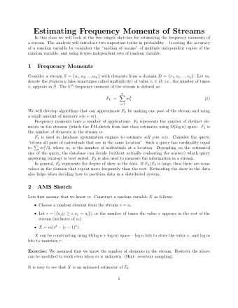
Frequency Moments Estimating Frequency Moments Anil Maheshwari Frequency Moments Definition Estimating F 0 Let A = ( a 1 , a 2 , . . . , a n ) be a stream, where elements are Algorithm from universe U = { 1 , . . . , u } . Let m i = # of elements in Correctness A that are equal to i . The k − th frequency moment Further Improvements u i , where 0 0 = 0 . m k F k = � Estimating F 2 i =1 Correctness Improving Variance An example for n = 19 and u = 7 Complexity A = (3 , 2 , 4 , 7 , 2 , 2 , 3 , 2 , 2 , 1 , 4 , 2 , 2 , 2 , 1 , 1 , 2 , 3 , 2) m 1 = 3 , m 2 = 10 , m 3 = 3 , m 4 = 2 , m 5 = 0 , m 6 = 0 , m 7 = 1

Example contd. Estimating Frequency Moments Anil Maheshwari Frequency Moments A = (3 , 2 , 4 , 7 , 2 , 2 , 3 , 2 , 2 , 1 , 4 , 2 , 2 , 2 , 1 , 1 , 2 , 3 , 2) and Estimating F 0 m 1 = m 3 = 3 , m 2 = 10 , m 4 = 2 , m 7 = 1 , m 5 = m 6 = 0 Algorithm 7 Correctness i = 3 0 + 10 0 + 3 0 + 2 0 + 0 0 + 0 0 + 1 0 = 5 m 0 F 0 = � Further i =1 Improvements (# of Distinct Elements in A ) Estimating F 2 7 Correctness i = 3 1 + 10 1 + 3 1 + 2 1 + 0 1 + 0 1 + 1 1 = 19 m 1 � F 1 = Improving i =1 Variance (# of Elements in A ) Complexity 7 i = 3 2 + 10 2 + 3 2 + 2 2 + 0 2 + 0 2 + 1 2 = 123 m 2 F 2 = � i =1 (Surprise Number)

Streaming Problem Estimating Frequency Moments Anil Maheshwari Frequency Moments Find frequency moments in a stream Estimating F 0 Algorithm Input: A stream A consisting of n elements from Correctness universe U = { 1 , . . . , u } . Further Output: Estimate Frequency Moments F k ’s for different Improvements values of k . Estimating F 2 Correctness Improving Our Task: Estimate F 0 and F 2 using sublinear space Variance Complexity Reference: The space complexity of estimating frequency moments by Noga Alon, Yossi Matias, and Mario Szegedy, Journal of Computer Systems and Science, 1999.

Estimating F 0 Estimating Frequency Moments Anil Maheshwari Frequency Moments Estimating F 0 Algorithm Computation of F 0 Correctness Further Input: Stream A = ( a 1 , a 2 , . . . , a n ) , where each Improvements a i ∈ U = { 1 , . . . , u } . Estimating F 2 Output: An estimate ˆ F 0 of number of distinct elements Correctness � ˆ � 1 F 0 ≥ 1 − 2 Improving F 0 in A such that Pr c ≤ F 0 ≤ c c for some Variance constant c using sublinear space. Complexity

Algorithm for Estimating F 0 Estimating Frequency Moments Anil Maheshwari Frequency Input: Stream A and a hash function h : U → U Moments Output: Estimate ˆ F 0 Estimating F 0 Algorithm Correctness Step 1: Initialize R := 0 Further Improvements Step 2: For each elements a i ∈ A do: Estimating F 2 Compute binary representation of h ( a i ) 1 Correctness Let r be the location of the rightmost 1 2 Improving Variance in the binary representation Complexity if r > R , R := r 3 Step 3: Return ˆ F 0 = 2 R Space Requirements = O (log u ) bits

Observations Estimating Frequency Moments Anil Maheshwari Let d to be smallest integer such that 2 d ≥ u ( d -bits are sufficient to represent numbers in U ) Frequency Moments Estimating F 0 Observation 1: Algorithm Pr ( rightmost 1 in h ( a i ) is at location ≥ r + 1) = 1 2 r Correctness Further Improvements Estimating F 2 Correctness Improving Variance Complexity

Observations contd. Estimating Frequency Moments Anil Maheshwari Observation 2: For a i � = a j , Pr ( rightmost 1 in 1 h ( a i ) ≥ r + 1 and rightmost 1 in h ( a j ) ≥ r + 1) = Frequency 2 2 r Moments Estimating F 0 Fix r ∈ { 1 , . . . , d } . ∀ x ∈ A , define indicator r.v: Algorithm Correctness � 1 , if the rightmost 1 is at location ≥ r + 1 in h ( x ) Further I r x = Improvements 0 , otherwise Estimating F 2 Let Z r = � I r Correctness x (sum is over distinct elements of A ) Improving Variance Observation 3: The following holds: Complexity x = 1) = 1 E [ I r x ] = Pr ( I r 2 r (see Observation 1) 1 x ] 2 = 1 2 ] − E [ I r 1 − 1 V ar [ I r x ] = E [ I r � � 2 x 2 r 2 r E [ Z r ] = F 0 3 2 r V ar [ Z r ] = F 0 1 1 − 1 ≤ F 0 � � 2 r = E [ Z r ] 4 2 r 2 r

Observations contd. Estimating Frequency Moments Anil Maheshwari Observation 4: If 2 r > cF 0 , Pr ( Z r > 0) < 1 c Frequency Proof: Markov’s Inequality states: Pr ( X ≥ a ) ≤ E [ X ] Moments a . Pr ( Z r > 0) = Pr ( Z r ≥ 1) ≤ E [ Z r ] = F 0 Estimating F 0 2 r < 1 c . Algorithm Correctness Observation 5: If c 2 r < F 0 , Pr ( Z r = 0) < 1 Further c Improvements Proof: Chebyshev’s Inequality states: Estimating F 2 Pr ( | X − E [ X ] | ≥ α ) ≤ V ar [ X ] . Correctness α 2 Note Pr ( Z r = 0) ≤ Pr ( | Z r − E [ Z r ] | ≥ E [ Z r ]) . Improving Variance Thus Pr ( Z r = 0) ≤ V ar [ Z r ] E [ Z r ] ≤ 2 r 1 F 0 < 1 E [ Z r ] 2 ≤ Complexity c

Observations contd. Estimating Frequency Moments Anil Maheshwari Observation 6: In our algorithm, we set ˆ F 0 = 2 R . Frequency � � c ≤ 2 R 1 ≥ 1 − 2 We have Pr F 0 ≤ c c . Moments Estimating F 0 Proof: From Observation 4, if 2 R > cF 0 , Pr ( Z r > 0) < 1 c . Algorithm From Observation 5, if c 2 R < F 0 , Pr ( Z r = 0) < 1 Correctness c . Further c , 2 R > cF 0 or c 2 R < F 0 . (Failure) Improvements With Pr ≤ 2 Estimating F 2 c ≤ 2 R Thus, with Pr ≥ 1 − 2 c , 1 Correctness F 0 ≤ c . (Success) Improving Variance Complexity

Improving success probability Estimating Frequency Moments Anil Maheshwari Execute the algorithm s times in parallel with independent hash functions. Frequency Moments Let R to the median value among these runs. Estimating F 0 Return ˆ Algorithm F 0 = 2 R . Correctness Claim: For c > 4 , there exists s = O (log 1 ǫ ) , ǫ > 0 , such Further Improvements ˆ that 1 F 0 c ≤ F 0 ≤ c with Pr ≥ 1 − ǫ and the algorithm uses Estimating F 2 O ( s log u ) bits. Correctness Improving Proof uses Chernoff Bounds: If r.v. X is sum of Variance independent identical indicator r.v. and 0 < δ < 1 , Complexity Pr ( X ≥ (1 + δ ) E [ X ]) ≤ e − δ 2 E [ X ] 3

Improving success probability contd. Estimating Frequency Moments Anil Maheshwari Define indicator r.v. X 1 , . . . , X s : Frequency Moments � c ≤ 2 Ri if success, i.e. 1 0 , F 0 ≤ c Estimating F 0 X i = 1 , otherwise Algorithm Correctness Note Further Improvements E [ X i ] = Pr ( X i = 1) ≤ 2 c = β < 1 1 2 Estimating F 2 s Correctness Let X = � X i = # Failures in s runs 2 Improving i =1 Variance E [ X ] ≤ sβ < s 3 Complexity 2 We apply Chernoff Bounds by setting s = O (log 1 ǫ ) . c ≤ 2 R Calculations will show that Pr ( 1 F 0 ≤ c ) ≥ 1 − ǫ

Estimating F 2 Estimating Frequency Moments Anil Maheshwari Frequency Moments Estimating F 0 Input: Stream A and hash function h : U → {− 1 , +1 } Algorithm u Output: Estimate ˆ m 2 F 2 of F 2 = � Correctness i i =1 Further Improvements Estimating F 2 Algorithm (Tug of War) Correctness Step 1: Initialize Y := 0 . Improving Variance Step 2: For each element x ∈ U , evaluate r x = h ( x ) . Complexity Step 3: For each element a i ∈ A , Y := Y + r a i Step 4: Return ˆ F 2 = Y 2

Observations Estimating Frequency Moments u Anil Maheshwari � Observation 1: Y = r i m i and E [ r i ] = 0 . i =1 Frequency Moments Estimating F 0 u Observation 2: E [ Y 2 ] = m 2 � i = F 2 Algorithm i =1 Correctness � u � 2 u u Further Y 2 = � = � � r i m i r i r j m i m j 1 Improvements i =1 i =1 j =1 Estimating F 2 � � Correctness u u E [ Y 2 ] = E � � r i r j m i m j 2 Improving Variance i =1 j =1 Complexity By Linearity of Expectation 3 u u E [ Y 2 ] = � � m i m j E [ r i r j ] i =1 j =1 By independence: E [ r i r j ] = E [ r i ] E [ r j ] . 4 u We have E [ Y 2 ] = m 2 � i = F 2 i =1

Observations contd. Estimating Frequency Moments Anil Maheshwari Frequency Moments √ Estimating F 0 | Y 2 − E [ Y 2 ] | ≥ 2 cE [ Y 2 ] ≤ 1 � � Observation 3: Pr c 2 for Algorithm any positive constant c . Correctness Further Proof Sketch: Improvements Estimating F 2 Chebyshev’s Inequality: 1 Correctness Pr ( | X − E [ X ] | ≥ α ) ≤ V ar [ X ] α 2 Improving Variance � � | Y 2 − E [ Y 2 ] | ≥ c ≤ 1 � V ar [ Y 2 ] Pr 2 c 2 Complexity V ar [ Y 2 ] = E [ Y 4 ] − E [ Y 2 ] 2 3

Observation 3 contd. Estimating Frequency Moments Anil Maheshwari Frequency E [ Y 4 ] � = E [ m i m j m k m l r i r j r k r l ] Moments Estimating F 0 i,j,k,l Algorithm � = m i m j m k m l E [ r i r j r k r l ] Correctness i,j,k,l Further u Improvements � � m 4 m 2 i m 2 = i + 6 Estimating F 2 j Correctness i =1 1 ≤ i<j ≤ u Improving Variance V ar [ Y 2 ] E [ Y 4 ] − E [ Y 2 ] 2 Complexity = � u � 2 u � � � m 4 m 2 i m 2 m 2 = i + 6 j − i i =1 1 ≤ i<j ≤ u i =1 � m 2 i m 2 = 4 j 1 ≤ i<j ≤ u