Estimating Frequency Moments of Streams In this class we will look - PDF document

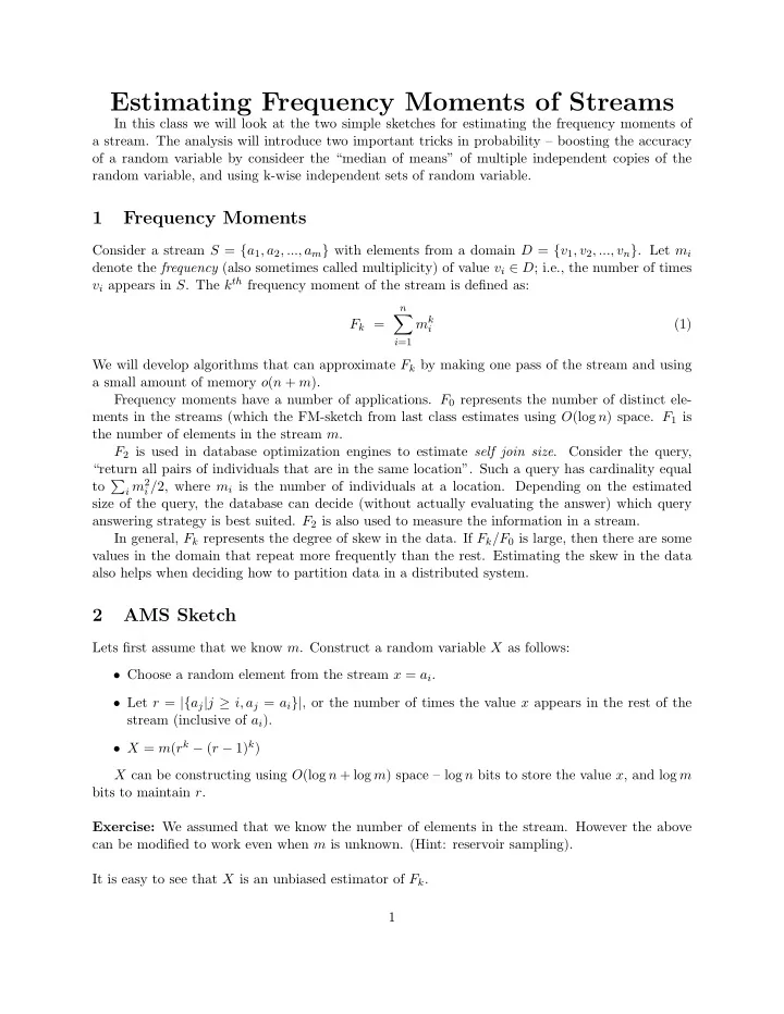
Estimating Frequency Moments of Streams In this class we will look at the two simple sketches for estimating the frequency moments of a stream. The analysis will introduce two important tricks in probability – boosting the accuracy of a random variable by consideer the “median of means” of multiple independent copies of the random variable, and using k-wise independent sets of random variable. 1 Frequency Moments Consider a stream S = { a 1 , a 2 , ..., a m } with elements from a domain D = { v 1 , v 2 , ..., v n } . Let m i denote the frequency (also sometimes called multiplicity) of value v i ∈ D ; i.e., the number of times v i appears in S . The k th frequency moment of the stream is defined as: n � m k F k = (1) i i =1 We will develop algorithms that can approximate F k by making one pass of the stream and using a small amount of memory o ( n + m ). Frequency moments have a number of applications. F 0 represents the number of distinct ele- ments in the streams (which the FM-sketch from last class estimates using O (log n ) space. F 1 is the number of elements in the stream m . F 2 is used in database optimization engines to estimate self join size . Consider the query, “return all pairs of individuals that are in the same location”. Such a query has cardinality equal i m 2 to � i / 2, where m i is the number of individuals at a location. Depending on the estimated size of the query, the database can decide (without actually evaluating the answer) which query answering strategy is best suited. F 2 is also used to measure the information in a stream. In general, F k represents the degree of skew in the data. If F k /F 0 is large, then there are some values in the domain that repeat more frequently than the rest. Estimating the skew in the data also helps when deciding how to partition data in a distributed system. 2 AMS Sketch Lets first assume that we know m . Construct a random variable X as follows: • Choose a random element from the stream x = a i . • Let r = |{ a j | j ≥ i, a j = a i }| , or the number of times the value x appears in the rest of the stream (inclusive of a i ). • X = m ( r k − ( r − 1) k ) X can be constructing using O (log n + log m ) space – log n bits to store the value x , and log m bits to maintain r . Exercise: We assumed that we know the number of elements in the stream. However the above can be modified to work even when m is unknown. (Hint: reservoir sampling). It is easy to see that X is an unbiased estimator of F k . 1

m 1 mE ( X | i th element in the stream was picked) � E ( X ) = i =1 n m i 1 E ( X | a i is the k th repetition of v j ) � � = m j =1 k =1 n m � 1 k + (2 k − 1 k ) + . . . + ( m k � � j − ( m j − 1) k ) = m j =1 n � m k = j = F k j =1 We now show how to use multiple such random variables X to estimate F k within ǫ relative error with high probability (1 − δ ). 2.1 Median of Means Suppose X is a random variable such that E ( X ) = µ and V ar ( X ) < cµ 2 , for some c > 0. Then, we can construct an estimator Z such that for all ǫ > 0 and δ > 0, E ( Z ) = E ( X ) = µ and P ( | Z − µ | > ǫµ ) < δ (2) by averaging s 1 = Θ( c/ǫ 2 ) independent copies of X , and then taking the median of s 2 = Θ(log(1 /δ )) such averages. Means: Let X 1 , . . . , X s 1 be s 1 copies of X . Let Y = 1 � i X i . Clearly, E ( Y ) = E ( X ) = µ . s 1 V ar ( X ) < cµ 2 1 V ar ( Y ) = s 1 s 1 V ar ( Y ) P ( | Y − µ | > ǫµ ) < by Chebyshev ǫ 2 µ 2 Therefore, if s 1 = 8 c ǫ 2 , then P ( | Y − µ | > ǫµ ) < 1 8 . Median of means: Now let Z be the median of s 2 copies of Y . Let W i be defined as follows: � 1 if | Y − µ | > ǫµ W i = 0 else From the previous result about Y , E ( W i ) = ρ < 1 8 . Therefore, E ( � i W i ) < s 2 / 8. Moreover, 2

whenever the median Z is outside the interval µ ± ǫ , � i W i > s 2 / 2. Therefore, � P ( | Z − µ | > ǫµ ) < P ( W i > s 2 / 2) i � � ≤ P ( | W i − E ( W i ) | > s 2 / 2 − s 2 ρ ) i i W i ) | > ( 1 � � = P ( | W i − E ( 2 ρ − 1) s 2 ρ ) i i � 2 � · s 2 ρ by Chernoff bounds 2 e − 1 1 2 ρ − 1 ≤ 3 · � 2 2 e − s 2 � 3 when ρ < 1 1 < 8 , ρ 2 ρ − 1 > 1 � 2 � Therefore, taking the median of s 2 = 3 log ensures that P ( | Z − µ | > ǫµ ) < δ . δ 2.2 Back to AMS We use the medians of means approach to boost the accuracy of the AMS random variable X . For that, we need to bound the variance of X by c · F 2 k . = E ( X 2 ) − E ( X ) 2 V ar ( X ) n m 2 � 1 2 k + (2 2 k − 1 2 k ) + . . . + ( m 2 k − ( m i − 1) 2 k � � E ( X 2 ) = i m i =1 When a > b > 0, we have k − 1 a k − b k = ( a − b )( � a j b k − 1 − j ) ≤ ( a − b )( ka k − 1 ) j =0 Therefore, k 1 2 k − 1 + ( k 2 k − 1 )(2 k − 1 k ) + . . . + km k − 1 ( m k � � E ( X 2 ) i − ( m i − 1) k ) ≤ m � � km 2 k − 1 + km 2 k − 1 + . . . + km 2 k − 1 ≤ m 1 2 n = kF 1 F 2 k − 1 Exercise: We can show that for all positive integers m 1 , m 2 , . . . , m n , � 2 �� � �� � �� ≤ n 1 − 1 m 2 k − 1 m k m i k i i i i i Therefore, we get that V ar ( X ) ≤ kn 1 − 1 k F 2 k . Hence, by using the median of means aggregation technique, we can estimate F k within a relative error of ǫ with probability at least (1 − δ ) using � 1 O ( kn 1 − 1 k 1 � ǫ 2 log ) independent estimators (each of which take O (log n + log m ) space. δ 3

3 A simpler sketch for F 2 √ n � 1 � Using the above analysis we can estimate F 2 using O ( ǫ 2 (log n + log m ) log ) bits. However, we δ can estimate F 2 using much smaller number of bits as follows. Suppose we have n independent uniform random variables x 1 , x 2 , . . . , x n each taking values in {− 1 , 1 } . (This requires n bits of memory, but we will show how to do this in O (log n ) bits in the next section). We compute a sketch as follows: • Compute r = � n i =1 x i · m i • Return r 2 as an estimate for F 2 . Note that r can be maintained as the new elements are seen in the stream by increasing/decreasing r by 1 depending on the sign of x i . Why does this work? � � � E ( r 2 ) x i m i ) 2 ] = m 2 i E [ x 2 = E [( i ] + 2 E [ x i x j m i m j ] i i i<j � m 2 = i = F 2 since x i , x j are independent, E ( x i x j ) is 0 i V ar ( r 2 ) E ( r 4 ) − F 2 = 2 � � � � E ( r 4 ) x i m i ) 2 ( x i m i ) 2 = E ( i i � � x 2 i m 2 x i x j m i m j )) 2 ] = E [(( i ) + (2 i i<j � � � � x 2 i m 2 i ) 2 ] + 4 E [( x i x j m i m j ) 2 ] + 4 E [( x 2 i m 2 = E [( i )( x i x j m i m j )] i i<j i i<j The last term is 0 since every pair of variables x i and x j are independent. Since x 2 i = 1, the first term is F 2 2 . � V ar ( r 2 ) E ( r 4 ) − F 2 x i x j m i m j ) 2 ] = 2 = 4 E [( i<j � � x 2 i x 2 j m 2 i m 2 = 4 E [ j ] + 4 E [ x i x j x k x l m i m j m k m l ] i<j i<j<k<l Again, the last term is 0 since every set of 4 random variables is independent of each other. Therefore, � V ar ( r 2 ) m 2 i m 2 j ≤ 2 F 2 = 4 2 i<j � 1 Therefore, by using the median of means method, we can estimate F 2 using Θ( 1 � ǫ 2 log ) indepen- δ dent estimates. However, the technique we presented needs O ( n ) random bits. We will reduce this to O (log n ) bits in the next section by using 4-wise independent random variables rather than fully independent random variables. 4