Classification or Regression? Regression Classification: want to - PowerPoint PPT Presentation
Classification or Regression? Regression Classification: want to learn a discrete target variable Machine Learning and Pattern Recognition Regression: want to learn a continuous target variable Linear regression,
Classification or Regression? Regression ◮ Classification: want to learn a discrete target variable Machine Learning and Pattern Recognition ◮ Regression: want to learn a continuous target variable ◮ Linear regression, linear-in-the-parameters models Chris Williams ◮ Linear regression is a conditional Gaussian model ◮ Maximum likelihood solution - ordinary least squares School of Informatics, University of Edinburgh ◮ Can use nonlinear basis functions ◮ Ridge regression September 2014 ◮ Full Bayesian treatment ◮ Reading: Murphy chapter 7 (not all sections needed), Barber (17.1, 17.2, 18.1.1) (All of the slides in this course have been adapted from previous versions by Charles Sutton, Amos Storkey, David Barber.) 1 / 24 2 / 24 One Dimensional Data Linear Regression 2.5 ◮ Simple example: one-dimensional linear regression. 2 ◮ Suppose we have data of the form ( x, y ) , and we believe the data should fol low a straight line: the data should have a 1.5 straight line fit of the form y = w 0 + w 1 x . ◮ However we also believe the target values y are subject to 1 measurement error, which we will assume to be Gaussian. So y = w 0 + w 1 x + η where η is a Gaussian noise term, mean 0 , variance σ 2 η . 0.5 0 −2 −1 0 1 2 3 3 / 24 4 / 24
Generated Data 2.5 2 1.5 1 0.5 Figure credit: http://jedismedicine.blogspot.co.uk/2014/01/ 0 ◮ Linear regression is just a conditional version of estimating a −2 −1 0 1 2 3 Gaussian (conditional on the input x ) 5 / 24 6 / 24 Multivariate Case Minimizing Squared Error ◮ Consider the case where we are interested in y = f ( x ) for D N dimensional x : y = w 0 + w 1 x 1 + . . . w D x D + η , where L ( w ) = − 1 ( y n − w T φ n ) 2 − N � 2 log(2 πσ 2 η ) η ∼ Gaussian (0 , σ 2 η ) . 2 σ 2 η n =1 ◮ Examples? Final grade depends on time spent on work for N � ( y n − w T φ n ) 2 − C 2 each tutorial. = − C 1 ◮ We set w = ( w 0 , w 1 , . . . w D ) T and introduce φ = (1 , x T ) T , n =1 then we can write y = w T φ + η instead where C 1 > 0 and C 2 don’t depend on w . Now ◮ This implies p ( y | φ , w ) = N ( y ; w T φ , σ 2 η ) ◮ Multiplying by a positive constant doesn’t change the ◮ Assume that training data is iid, i.e., maximum p ( y 1 , . . . y N | x 1 , . . . , x N , w ) = � N n =1 p ( y n | x n , w ) ◮ Adding a constant doesn’t change the maximum. ◮ � N n =1 ( y n − w T φ n ) 2 is the sum of squared errors made if you ◮ Given data { ( x n , y n ) , n = 1 , 2 , . . . , N } , the log likelihood is use w L ( w ) = log P ( y 1 . . . y N | x 1 . . . x N , w ) So maximizing the likelihood is the same as minimizing the total N squared error of the linear predictor. = − 1 ( y n − w T φ n ) 2 − N � 2 log(2 πσ 2 η ) 2 σ 2 So you don’t have to believe the Gaussian assumption. You can η n =1 simply believe that you want to minimize the squared error. 7 / 24 8 / 24
Maximum Likelihood Solution I Maximum Likelihood Solution II ◮ Setting the derivatives to zero to find the minimum gives Φ T Φ ˆ ◮ Write Φ = ( φ 1 , φ 2 , . . . , φ N ) T , and y = ( y 1 , y 2 , . . . , y N ) T w = Φ T y ◮ Φ is called the design matrix , has N rows, one for each ◮ This means the maximum likelihood ˆ w is given by example w = (Φ T Φ) − 1 Φ T y ˆ L ( w ) = − 1 ( y − Φ w ) T ( y − Φ w ) − C 2 2 σ 2 The matrix (Φ T Φ) − 1 Φ T is called the pseudo-inverse . η ◮ Ordinary least squares (OLS) solution for w ◮ Take derivatives of the log likelihood: ◮ MLE for the variance ∇ w L ( w ) = − 1 Φ T (Φ w − y ) σ 2 N η η = 1 � ( y n − w T φ n ) 2 σ 2 ˆ N n =1 i.e. the average of the squared residuals 9 / 24 10 / 24 Generated Data Nonlinear regression 2.5 ◮ All this just used φ . 2 ◮ We chose to put the x values in φ , but we could have put anything in there, including nonlinear transformations of the x 1.5 values. ◮ In fact we can choose any useful form for φ so long as the final 1 derivatives are linear wrt w . We can even change the size. 0.5 ◮ We already have the maximum likelihood solution in the case of Gaussian noise: the pseudo-inverse solution. 0 ◮ Models of this form are called general linear models or linear-in-the-parameters models. −0.5 −2 −1 0 1 2 3 The black line is the maximum likelihood fit to the data. 11 / 24 12 / 24
Example:polynomial fitting Dimensionality issues ◮ Model y = w 1 + w 2 x + w 2 x 2 + w 4 x 3 . ◮ Set φ = (1 , x, x 2 , x 3 ) T and w = ( w 1 , w 2 , w 3 , w 4 ) . ◮ Can immediately write down the ML solution: ◮ How many radial basis functions do we need? w = (Φ T Φ) − 1 Φ T y , where Φ and y are defined as before. ◮ Suppose we need only three per dimension ◮ Could use any features we want: e.g. features that are only ◮ Then we would need 3 D for a D -dimensional problem active in certain local regions (radial basis functions, RBFs). ◮ This becomes large very fast: this is commonly called the curse of dimensionality ◮ Gaussian processes (see later) can help with these issues Figure credit: David Barber, BRML Fig 17.6 13 / 24 14 / 24 Higher dimensional outputs Adding a Prior ◮ Put prior over parameters, e.g., p ( y | φ , w ) = N ( y ; w T φ , σ 2 η ) p ( w ) = N ( w ; 0 , τ 2 I ) ◮ I is the identity matrix ◮ The log posterior is ◮ Suppose the target values are vectors. ◮ Then we introduce different w i for each y i . N 1 ( y n − w T φ n ) 2 − N � 2 log(2 πσ 2 ) log p ( w |D ) = const − ◮ Then we can do regression independently in each of those 2 σ 2 η n =1 cases. 1 − D 2 τ 2 w T w 2 log(2 πτ 2 ) − � �� � penalty on large weights ◮ MAP solution can be computed analytically. Derivation almost the same as with MLE (where λ = σ 2 η /τ 2 ) w MAP = (Φ T Φ + λI ) − 1 Φ T y This is called ridge regression 15 / 24 16 / 24
Effect of Ridge Regression Effect of Ridge Regression (Graphic) ◮ Collecting constant terms from log posterior on last slide N ln lambda −20.135 ln lambda −8.571 log p ( w |D ) = const − 1 1 � ( y n − w T φ n ) 2 − 20 20 2 τ 2 w T w 2 σ 2 15 η 15 n =1 � �� � || w || 2 10 2 . penalty term 10 5 ◮ This is called ℓ 2 regularization or weight decay . The second 5 0 term is the squared Euclidean (also called ℓ 2 ) norm of w . 0 −5 ◮ The idea is to reduce overfitting by forcing the function to be −5 −10 simple. The simplest possible function is constant w = 0 , so −10 −15 0 5 10 15 20 0 5 10 15 20 encourage ˆ w to be closer to that. ◮ τ is a parameter of the method. Trades off between how well Figure credit: Murphy Fig 7.7 you fit the training data and how simple the method is. Most Degree 14 polynomial fit with and without regularization commonly set via cross validation. ◮ Regularization is a general term for adding a “second term” to an objective function to encourage simple models. 17 / 24 18 / 24 Why Ridge Regression Works (Graphic) Bayesian Regression u 2 ◮ Bayesian regression model p ( y | φ , w ) = N ( y ; w T φ , σ 2 η ) u 1 p ( w ) = N ( w ; 0 , τ 2 I ) ML Estimate MAP Estimate ◮ Possible to compute the posterior distribution analytically, because linear Gaussian models are jointly Gaussian (see Murphy § 7.6.1 for details) prior mean p ( w | Φ , y , σ 2 η ) ∝ p ( w ) p ( y | Φ , σ 2 η ) = N ( w | w N , V N ) w N = 1 V N Φ T y σ 2 η η /τ 2 I + Φ T Φ) − 1 V N = σ 2 η ( σ 2 Figure credit: Murphy Fig 7.9 19 / 24 20 / 24
Making predictions Example of Bayesian Regression likelihood prior/posterior data space 1 1 W1 y 0 0 −1 −1 −1 0 1 −1 0 1 ◮ For a new test point x ∗ with corresponding feature vector φ ∗ , W0 x 1 1 1 we have that W1 W1 y f ( x ∗ ) = w T φ ∗ + η 0 0 0 −1 −1 −1 −1 0 1 −1 0 1 −1 0 1 where w ∼ N ( w N , V N ) . W0 W0 x ◮ Hence 1 1 1 W1 W1 y 0 0 0 N φ ∗ , ( φ ∗ ) T V N φ ∗ + σ 2 p ( y ∗ | x ∗ , D ) ∼ N ( w T η ) −1 −1 −1 −1 0 1 −1 0 1 −1 0 1 W0 W0 x 1 1 1 W1 W1 y 0 0 0 −1 −1 −1 −1 0 1 −1 0 1 −1 0 1 W0 W0 x Figure credit: Murphy Fig 7.11 21 / 24 22 / 24 Another Example Summary plugin approximation (MLE) Posterior predictive (known variance) 60 80 prediction prediction training data training data 70 50 60 40 50 40 30 30 20 20 10 ◮ Linear regression is a conditional Gaussian model 10 0 0 −10 −8 −6 −4 −2 0 2 4 6 8 −8 −6 −4 −2 0 2 4 6 8 ◮ Maximum likelihood solution - ordinary least squares MLE Bayes ◮ Can use nonlinear basis functions functions sampled from plugin approximation to posterior functions sampled from posterior 50 100 45 ◮ Ridge regression 80 40 35 60 ◮ Full Bayesian treatment 30 25 40 20 20 15 10 0 5 0 −20 −8 −6 −4 −2 0 2 4 6 8 −8 −6 −4 −2 0 2 4 6 8 MLE samples Bayes samples Figure credit: Murphy Fig 7.12 Fitting a quadratic. Notice how the error bars get larger further away from training data 23 / 24 24 / 24
Recommend
More recommend
Explore More Topics
Stay informed with curated content and fresh updates.



![Classification Image Classification Set of predefined categories [eg: table, apple, dog, giraffe]](https://c.sambuz.com/743996/classification-s.webp)
