IAML: Decision Trees Chris Williams and Victor Lavrenko School of - PowerPoint PPT Presentation
IAML: Decision Trees Chris Williams and Victor Lavrenko School of Informatics Semester 1 1 / 17 Outline Decision trees: the idea Examples Top-down induction of decision trees Entropy Information gain Overfitting and
IAML: Decision Trees Chris Williams and Victor Lavrenko School of Informatics Semester 1 1 / 17
Outline ◮ Decision trees: the idea ◮ Examples ◮ Top-down induction of decision trees ◮ Entropy ◮ Information gain ◮ Overfitting and pruning ◮ Reading off rules from decision trees ◮ Reading: W & F sec 4.3, and 6.1 (only numeric attributes, pruning sections required) 2 / 17
Decision Trees ◮ The idea is to partition input space into a disjoint set of regions and to use a very simple predictor for each region ◮ For classification simply predict the most frequent class in the region ◮ We could estimate class probabilities by the relative frequencies of training data in the region ◮ For regression the predicted output is just the mean of the training data in the region 3 / 17
Example 1 Continuous inputs x 2 E x 1 > θ 1 θ 3 B x 2 � θ 2 x 2 > θ 3 C D θ 2 x 1 � θ 4 A x 1 θ 1 θ 4 A B C D E Figure credit: Chris Bishop, PRML 4 / 17
Example 2 Discrete inputs Outlook Sunny Overcast Rain Wind Humidity Yes High Normal Strong Weak No Yes No Yes Figure credit: Tom Mitchell, 1997 5 / 17
Play Tennis training data Day Outlook Temperature Humidity Wind PlayTennis D1 Sunny Hot High Weak No D2 Sunny Hot High Strong No D3 Overcast Hot High Weak Yes D4 Rain Mild High Weak Yes D5 Rain Cool Normal Weak Yes D6 Rain Cool Normal Strong No D7 Overcast Cool Normal Strong Yes D8 Sunny Mild High Weak No D9 Sunny Cool Normal Weak Yes D10 Rain Mild Normal Weak Yes D11 Sunny Mild Normal Strong Yes D12 Overcast Mild High Strong Yes D13 Overcast Hot Normal Weak Yes D14 Rain Mild High Strong No 6 / 17
Top-Down Induction of Decision Trees ID3 algorithm (Quinlan, 1986) Main loop: 1. A ← the “best” decision attribute for next node 2. Assign A as decision attribute for node 3. For each value of A , create new descendant of node 4. Sort training examples to leaf nodes 5. If training examples perfectly classified, Then STOP , Else iterate over new leaf nodes 7 / 17
Decision tree representation ◮ Each internal node tests an attribute ◮ Each branch corresponds to attribute value ◮ Each leaf node makes a prediction 8 / 17
Entropy ◮ S is a sample of training examples ◮ p ⊕ is the proportion of positive examples in S ◮ p ⊖ is the proportion of negative examples in S ◮ Entropy measures the impurity of S Entropy ( S ) ≡ H ( S ) ≡ − p ⊕ log 2 p ⊕ − p ⊖ log 2 p ⊖ bits ◮ H ( S ) = 0 if sample is pure (all + or all -), H ( S ) = 1 bit if p ⊕ = p ⊖ = 0 . 5 9 / 17
Information Gain ◮ Gain ( S , A ) = expected reduction in entropy due to sorting on A | S v | � Gain ( S , A ) ≡ Entropy ( S ) − | S | Entropy ( S v ) v ∈ Values ( A ) ◮ Information gain is also called the mutual information between A and the labels of S ◮ Example: In the play tennis sample there are 14 examples, 9 +, 5 -, written as [9,5]. Splitting on outlook we get [2,3] (for sunny), [4,0] (for overcast), [3,2] (for rainy). Gain ( S , Outlook ) = H ([ 9 , 5 ]) − 5 14 H ([ 2 , 3 ]) − 4 14 H ([ 4 , 0 ]) − 5 14 H ([ 3 , 2 ]) = 0 . 247 bits 10 / 17
Overfitting in Decision Tree Learning ◮ Overfitting can occur with noisy training examples, and also when small numbers of examples are associated with leaf nodes ( → coincidental or accidental regularities) 0.9 0.85 0.8 0.75 Accuracy 0.7 0.65 0.6 On training data On test data 0.55 0.5 0 10 20 30 40 50 60 70 80 90 100 Size of tree (number of nodes) Figure credit: Tom Mitchell, 1997 11 / 17
Avoiding Overfitting ◮ Stop growing when data split not statistically significant ◮ Grow full tree, then post-prune ◮ The latter strategy is usually used, based on the performance on a validation set ◮ Subtree replacement pruning (W & F , § 6.1) Do until further pruning is harmful: 1. Evaluate impact on validation set of pruning each possible node (plus those below it) 2. Greedily remove the one that most improves validation set accuracy 12 / 17
Fitting this into the general structure for learning algorithms: ◮ Define the task : classification, discriminative ◮ Decide on the model structure : decision tree ◮ Decide on the score function : information gain at each node, overall objective function is unclear ◮ Decide on optimization/search method : greedy search from simple to complex, guided by information gain heuristic. Other comments: ◮ Preference for short trees, and for those with high information gain attributes near the root ◮ Bias is a preference for some hypotheses, rather than a restriction of hypothesis space 13 / 17
Alternative Measures for Selecting Attributes ◮ Problem: if an attribute has many values, Gain will select it ◮ Example: use of dates in database entries ◮ One approach: use GainRatio instead Gain ( S , A ) GainRatio ( S , A ) ≡ SplitInformation ( S , A ) c | S i | | S i | � SplitInformation ( S , A ) ≡ − | S | log 2 | S | i = 1 where S i is subset of S for which A has value v i 14 / 17
Reading off Rules from Decision Trees Outlook Sunny Overcast Rain Wind Humidity Yes High Normal Strong Weak No Yes No Yes Figure credit: Tom Mitchell, 1997 ( Outlook = Sunny ∧ Humidity = Normal ) ∨ ( Outlook = Overcast ) ∨ ( Outlook = Rain ∧ Wind = Weak ) 15 / 17
Further Issues ◮ Dealing with continuous-valued attributes—create a split, e.g. ( Temperature > 72 . 3 ) = t , f . Split point can be optimized (W & F § 6.1) ◮ For regression, can use linear regression at leaves → model trees (discussed in W & F § 6.5, not examinable) ◮ Can handle training examples with missing data (discussed in W & F § 6.1, not examinable) ◮ Decision trees can easily ignore irrelevant variables ◮ CART (classification and regression trees, Breiman et al, 1984) from statistics ◮ ID3 and later C4.5 from Ross Quinlan (1986, 1993) 16 / 17
Summary ◮ ID3 algorithm grows decision trees from the root downwards, greedily selecting the next best attribute for each new decision branch ◮ ID3 searches a complete hypothesis space, using a preference bias for smaller trees with higher information gain close to the root ◮ The overfitting problem can be tackled using post-pruning 17 / 17
Recommend
More recommend
Explore More Topics
Stay informed with curated content and fresh updates.
