Outline IAML: Basic Probability and Estimation Random Variables - PowerPoint PPT Presentation

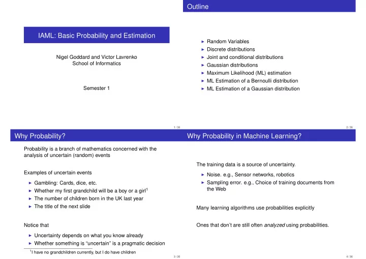
Outline IAML: Basic Probability and Estimation ◮ Random Variables ◮ Discrete distributions ◮ Joint and conditional distributions Nigel Goddard and Victor Lavrenko School of Informatics ◮ Gaussian distributions ◮ Maximum Likelihood (ML) estimation ◮ ML Estimation of a Bernoulli distribution ◮ ML Estimation of a Gaussian distribution Semester 1 1 / 36 2 / 36 Why Probability? Why Probability in Machine Learning? Probability is a branch of mathematics concerned with the analysis of uncertain (random) events The training data is a source of uncertainty. Examples of uncertain events ◮ Noise. e.g., Sensor networks, robotics ◮ Sampling error. e.g., Choice of training documents from ◮ Gambling: Cards, dice, etc. the Web ◮ Whether my first grandchild will be a boy or a girl 1 ◮ The number of children born in the UK last year ◮ The title of the next slide Many learning algorithms use probabilities explicitly Notice that Ones that don’t are still often analyzed using probabilities. ◮ Uncertainty depends on what you know already ◮ Whether something is “uncertain” is a pragmatic decision 1 I have no grandchildren currently, but I do have children 3 / 36 4 / 36

Random Variables Discrete Random Variables Random variables (RVs) can be discrete or continuous . 0.14 ◮ The set of all possible outcomes of an experiment is called 0.12 the sample space , denoted by Ω 0.1 ◮ Events are subsets of Ω (often singletons) 0.08 ◮ A random variable takes on values from a collection of 0.06 mutually exclusive and collectively exhaustive states, where each state corresponds to some event 0.04 ◮ A random variable X is a map from the sample space to 0.02 the set of states 0 5 10 15 20 25 30 35 ◮ Examples of variables ◮ Use capital letters to denote random variables and lower ◮ Colour of a car blue , green , red ◮ Number of children in a family 0 , 1 , 2 , 3 , 4 , 5 , 6 , > 6 case letters to denote values that they take, e.g. p ( X = x ) . ◮ Toss two coins, let X = ( number of heads ) 2 . What values Often shortened to p ( x ) . can X take? ◮ p ( x ) is called a probability mass function . ◮ For discrete RVs: � x p ( x ) = 1. 5 / 36 6 / 36 Examples: Discrete Distributions Frequency ◮ Example 1: Coin toss: 0 or 1 12 0.14 ◮ Example 2: Have data for the number of characters in 10 0.12 names of 88 people submitting tutorial requests: 0.1 8 9 10 10 11 11 11 11 11 11 12 12 12 12 12 12 0.08 count 6 12 12 12 13 13 13 13 13 13 13 13 13 13 13 0.06 14 14 14 14 14 14 14 14 14 14 14 15 15 15 4 0.04 15 15 15 15 15 15 15 15 15 16 16 16 16 16 2 16 16 17 17 17 17 17 18 18 19 19 19 19 20 0.02 20 20 20 20 21 21 21 21 21 22 22 22 24 25 0 5 10 15 20 25 30 35 0 number of characters in name 5 10 15 20 25 30 35 27 27 30 frequency normalized frequency ◮ Example 3: Third word on this slide. 7 / 36 8 / 36

Joint distributions Marginal Probabilities ◮ Suppose X and Y are two random variables. X takes on The sum rule the value yes if the word “password” occurs in an email, � p ( X ) = p ( X , Y ) and no if this word is not present. Y takes on the values of y ham and spam ◮ This example relates to “spam filtering” for email e.g. P ( X = yes ) = ? Y = ham Y = spam X = yes 0 . 01 0 . 25 X = no 0 . 49 0 . 25 ◮ Notation p ( X = yes , Y = ham ) = 0 . 01 9 / 36 10 / 36 Marginal Probabilities Conditional Probability ◮ Let X and Y be two disjoint subsets of variables, such that p ( Y = y ) > 0. Then the conditional probability distribution The sum rule (CPD) of X given Y = y is given by � p ( X ) = p ( X , Y ) y p ( X = x | Y = y ) = p ( x | y ) = p ( x , y ) p ( y ) e.g. P ( X = yes ) = ? ◮ Gives us the product rule Similarly: � p ( Y ) = p ( X , Y ) p ( X , Y ) = p ( Y ) p ( X | Y ) = p ( X ) p ( Y | X ) x ◮ Example : In the ham/spam example, what is e.g. P ( Y = ham ) = ? p ( X = yes | Y = ham ) ? ◮ � x p ( X = x | Y = y ) = 1 for all y 11 / 36 12 / 36

Bayes’ Rule Independence ◮ Independence means that one variable does not affect another, X is (marginally) independent of Y if ◮ From the product rule, p ( X | Y ) = P ( X ) p ( Y | X ) = p ( X | Y ) p ( Y ) ◮ This is equivalent to saying p ( X ) p ( X , Y ) = p ( X ) p ( Y ) ◮ From the sum rule the denominator is (can show this from definition of conditional probability) � p ( X ) = p ( X | Y ) p ( Y ) ◮ X 1 is conditionally independent of X 2 given Y if y p ( X 1 | X 2 , Y ) = p ( X 1 | Y ) ◮ Say that Y denotes a class label, and X an observation. Then p ( Y ) is the prior distribution for a label, and p ( Y | X ) is (i.e., once I know Y , knowing X 2 does not provide the posterior distribution for Y given a datapoint x . additional information about X 1 ) ◮ These are different things. Conditional independence does not imply marginal independence, nor vice versa. 13 / 36 14 / 36 Continuous Random Variables Mean, variance Suppose we want random values in R . Example: sample measurements p(x) For a continuous RV � � 70 σ 2 = 0 10 30 40 50 60 20 ( x − µ ) 2 p ( x ) dx µ = xp ( x ) dx x (Haggis length in cm) ◮ Formally, a continuous random variable X is a map ◮ µ is the mean X : Σ → R . ◮ σ 2 is the variance ◮ In continuous case, p ( x ) is called a density function ◮ Get the probability Pr { X ∈ [ a , b ] } by integration ◮ For numerical discrete variables, convert integrals to sums � b ◮ Also written: EX = � xp ( x ) dx for the mean and Pr { X ∈ [ a , b ] } = p ( x ) dx ◮ VX = E ( X − µ ) 2 = � ( x − µ ) 2 p ( x ) dx for the variance a ◮ Always true: p ( x ) > 0 for all x and � p ( x ) dx = 1 ( cf discrete case). ◮ Bayes’ rule, conditional densities, joint densities work exactly as in the discrete case. 15 / 36 16 / 36

Example: Uniform Distribution Quiz Question Let X be a continuous random variable on [ 0 , N ] such that “all points are equally likely.” This is called the uniform distribution on [ 0 , N ] . Its density is ◮ Let X be a continuous random variable with density p . 0.25 � ◮ Need it be true that p ( x ) < 1? 1 if x ∈ [ 0 , N ] N p ( x ) = p(x) 0.20 0 otherwise 0.15 0 1 2 3 4 5 X What is EX ? What is VX ? 17 / 36 18 / 36 Example: Another Uniform Distribution Gaussian distribution Imagine that I am throwing darts on a dartboard. 0.5 1 ◮ The most common (and most easily analyzed) distribution for continuous quantities is the Gaussian distribution. ◮ Gaussian distribution is often a reasonable model for many quantities due to various central limit theorems ◮ Gaussian is also called the normal distribution Let X be the x -position of the dart I throw, and Y be the y position. Assuming that the dart is equally likely to land anywhere on the board: 1. What is the probability it will land in the inner circle? 2. What what is the joint density of X and Y ? 19 / 36 20 / 36

Definition Plot 0.4 0.35 0.3 0.25 ◮ The one-dimensional Gaussian distribution is given by 0.2 − ( x − µ ) 2 1 � � 0.15 p ( x | µ, σ 2 ) = N ( x ; µ, σ 2 ) = √ 2 πσ 2 exp 2 σ 2 0.1 0.05 ◮ µ is the mean of the Gaussian and σ 2 is the variance . 0 −5 −4 −3 −2 −1 0 1 2 3 4 5 ◮ If µ = 0 and σ 2 = 1 then N ( x ; µ, σ 2 ) is called a standard Gaussian. ◮ This is a standard one dimensional Gaussian distribution. ◮ All Gaussians have the same shape subject to scaling and displacement. ◮ If x is distributed N ( x ; µ, σ 2 ) , then y = ( x − µ ) /σ is distributed N ( y ; 0 , 1 ) . 21 / 36 22 / 36 Normalization Bivariate Gaussian I ◮ Remember all distributions must integrate to one. The √ 2 πσ 2 is called a normalization constant - it ensures this is ◮ Let X 1 ∼ N ( µ 1 , σ 2 1 ) and X 2 ∼ N ( µ 2 , σ 2 2 ) the case. ◮ If X 1 and X 2 are independent ◮ Hence tighter Gaussians have higher peaks: � ( x 1 − µ 1 ) 2 + ( x 2 − µ 2 ) 2 1 � − 1 �� p ( x 1 , x 2 ) = 2 ) 1 / 2 exp 0.4 2 π ( σ 2 1 σ 2 σ 2 σ 2 2 1 2 0.35 � x 1 � µ 1 � σ 2 0.3 � � � 0 ◮ Let x = 1 , µ = , Σ = σ 2 x 2 µ 2 0 0.25 2 0.2 1 � − 1 �� 0.15 � ( x − µ ) T Σ − 1 ( x − µ ) p ( x ) = 2 π | Σ | 1 / 2 exp 2 0.1 0.05 0 −8 −6 −4 −2 0 2 4 6 8 23 / 36 24 / 36

Bivariate Gaussian II ◮ Covariance 1 ◮ Σ is the covariance 0.8 matrix 0.6 0.4 Σ = E [( x − µ )( x − µ ) T ] 0.2 0 2 Σ ij = E [( x i − µ i )( x j − µ j )] 1 2 1 0 0 −1 −1 ◮ Example: plot of weight −2 −2 vs height for a population 25 / 36 26 / 36 Multivariate Gaussian Inverse Problem: Estimating a Distribution ◮ p ( x ∈ R ) = � R p ( x ) d x ◮ Multivariate Gaussian ◮ But what if we don’t know the underlying distribution? 1 � − 1 � ◮ Want to learn a good distribution that fits the data we do 2 ( x − µ ) T Σ − 1 ( x − µ ) p ( x ) = ( 2 π ) d / 2 | Σ | 1 / 2 exp have ◮ How is goodness measured? ◮ Σ is the covariance matrix ◮ Given some distribution, we can ask how likely it is to have Σ ij = E [( x i − µ i )( x j − µ j )] generated the data ◮ In other words what is the probability (density) of this Σ = E [( x − µ )( x − µ ) T ] particular data set given the distribution ◮ Σ is symmetric ◮ A particular distribution explains the data better if the data ◮ Shorthand x ∼ N ( µ , Σ) is more probable under that distribution ◮ For p ( x ) to be a density, Σ must be positive definite ◮ Σ has d ( d + 1 ) / 2 parameters, the mean has a further d 27 / 36 28 / 36