Quick Tour of Basic Probability Theory and Linear Algebra CS224w: - PowerPoint PPT Presentation

Quick Tour of Basic Probability Theory and Linear Algebra Quick Tour of Basic Probability Theory and Linear Algebra CS224w: Social and Information Network Analysis Fall 2011

Quick Tour of Basic Probability Theory and Linear Algebra Basic Probability Theory Basic Probability Theory

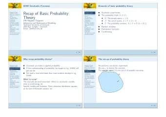
Quick Tour of Basic Probability Theory and Linear Algebra Basic Probability Theory Outline Definitions and theorems: independence, Bayes,. . . Random variables: pdf, expectation, variance, typical distributions,. . . Bounds: Markov, Chebyshev and Chernoff Method of indicators Multi-dimensional random variables: joint distribution, covariance,. . . Maximum likelihood estimation Convergence: Central limit theorem and interesting limits

Quick Tour of Basic Probability Theory and Linear Algebra Basic Probability Theory Elements of Probability Definition: Sample Space Ω : Set of all possible outcomes Event Space F : A family of subsets of Ω Probability Measure: Function P : F → R with properties: 1 P ( A ) ≥ 0 ( ∀ A ∈ F ) 2 P (Ω) = 1 3 A i ’s disjoint, then P ( � i A i ) = � i P ( A i ) Sample spaces can be discrete (rolling a die) or continuous (wait time in line)

Quick Tour of Basic Probability Theory and Linear Algebra Basic Probability Theory Conditional Probability and Independence Conditional probability: For events A , B : P ( A | B ) = P ( A � B ) P ( B ) Intuitively means “probability of A when B is known” Independence A, B independent if P ( A | B ) = P ( A ) or equivalently: P ( A � B ) = P ( A ) P ( B ) Beware of intuition: roll two dies ( x a and x b ), outcomes { x a = 2 } and { x a + x b = k } are independent if k = 7, but not otherwise!

Quick Tour of Basic Probability Theory and Linear Algebra Basic Probability Theory Basic laws and bounds Union bound: since P ( A ∪ B ) = P ( A ) + P ( B ) − P ( A ∩ B ) , we have P ( A i ) ≤ P ( A i ) � � i i i A i = Ω , then Law of total probability: if � P ( B ) = P ( A i ∩ B ) = P ( A i ) P ( B | A i ) � � i i Chain rule: P ( A 1 , A 2 , . . . , A N ) = P ( A 1 ) P ( A 2 | A 1 ) P ( A 3 | A 1 , A 2 ) · · · P ( A N | A 1 , . . . , A N − 1 ) Bayes rule: P ( A | B ) = P ( B | A ) P ( A ) P ( B ) (several versions)

Quick Tour of Basic Probability Theory and Linear Algebra Basic Probability Theory Random Variables and Distributions A random variable X is a function X : Ω → R Example: Number of heads in 20 tosses of a coin Probabilities of events associated with random variables defined based on the original probability function. e.g., P ( X = k ) = P ( { ω ∈ Ω | X ( ω ) = k } ) Cumulative Distribution Function (CDF) F X : R → [ 0 , 1 ] : F X ( x ) = P ( X ≤ x ) ( X discrete) Probability Mass Function (pmf): p X ( x ) = P ( X = x ) ( X continuous) Probability Density Function (pdf): f X ( x ) = dF X ( x ) / dx

Quick Tour of Basic Probability Theory and Linear Algebra Basic Probability Theory Properties of Distribution Functions CDF: 0 ≤ F X ( x ) ≤ 1 F X monotone increasing, with lim x →−∞ F X ( x ) = 0, lim x →∞ F X ( x ) = 1 pmf: 0 ≤ p X ( x ) ≤ 1 x p X ( x ) = 1 � x ∈ A p X ( x ) = p X ( A ) � pdf: f X ( x ) ≥ 0 � ∞ −∞ f X ( x ) dx = 1 x ∈ A f X ( x ) dx = P ( X ∈ A ) �

Quick Tour of Basic Probability Theory and Linear Algebra Basic Probability Theory Expectation and Variance Assume random variable X has pdf f X ( x ) , and g : R → R . Then � ∞ E [ g ( X )] = g ( x ) f X ( x ) dx −∞ for discrete X , E [ g ( X )] = � x g ( x ) p X ( x ) Expectation is linear: for any constant a ∈ R , E [ a ] = a E [ ag ( X )] = aE [ g ( X )] E [ g ( X ) + h ( X )] = E [ g ( X )] + E [ h ( X )] Var [ X ] = E [( X − E [ X ]) 2 ] = E [ X 2 ] − E [ X ] 2

Quick Tour of Basic Probability Theory and Linear Algebra Basic Probability Theory Conditional Expectation E [ g ( X , Y ) | Y = a ] = � x g ( x , a ) p X | Y = a ( x ) (similar for continuous random variables) Iterated expectation: E [ g ( X , Y )] = E a [ E [ g ( X , Y ) | Y = a ]] Often useful in practice. Example: number of heads in N flips of a coin with random bias p ∈ [ 0 , 1 ] with pdf f p ( x ) = 2 ( 1 − x ) is N 3

Quick Tour of Basic Probability Theory and Linear Algebra Basic Probability Theory Some Common Random Variables � p x=1 , X ∼ Bernoulli ( p ) (0 ≤ p ≤ 1): p X ( x ) = 1 − p x=0 . X ∼ Geometric ( p ) (0 ≤ p ≤ 1): p X ( x ) = p ( 1 − p ) x − 1 � a ≤ x ≤ b , 1 b − a X ∼ Uniform ( a , b ) ( a < b ): f X ( x ) = 0 otherwise . 2 σ 2 ( x − µ ) 2 1 X ∼ Normal ( µ, σ 2 ) : f X ( x ) = 2 πσ e − 1 √

Quick Tour of Basic Probability Theory and Linear Algebra Basic Probability Theory Binomial distribution Combinatorics: consider a bag with n different balls number of different ordered subsets with k elements: n ( n − 1 ) · · · ( n − k + 1 ) number of different unordered subsets with k elements: n ! � � n = k !( n − k )! k X ∼ Binomial ( n , p ) ( n > 0 , 0 ≤ p ≤ 1): � n � p x ( 1 − p ) n − x p X ( x ) = x

Quick Tour of Basic Probability Theory and Linear Algebra Basic Probability Theory Method of indicators Goal: find expected number of successes out of N trials Method: define an indicator (Bernoulli) random variable for each trial, find expected value of the sum Examples: Bowl with N spaghetti strands. Keep picking ends and joining. Expected number of loops? N drunk sailors pass out on random bunks. Expected number on their own?

Quick Tour of Basic Probability Theory and Linear Algebra Basic Probability Theory Some Useful Inequalities Markov’s Inequality: X random variable, and a > 0. Then: P ( | X | ≥ a ) ≤ E [ | X | ] a Chebyshev’s Inequality: If E [ X ] = µ , Var ( X ) = σ 2 , k > 0, then: Pr ( | X − µ | ≥ k σ ) ≤ 1 k 2 Chernoff bound: Let X 1 , . . . , X n independent Bernoulli with P ( X i = 1 ) = p i . Denoting µ = E [ � n i = 1 X i ] = � n i = 1 p i , n e δ � µ � P ( X i ≥ ( 1 + δ ) µ ) ≤ � ( 1 + δ ) 1 + δ i = 1 for any δ . Multiple variants of Chernoff-type bounds exist, which can be useful in different settings

Quick Tour of Basic Probability Theory and Linear Algebra Basic Probability Theory Multiple Random Variables and Joint Distributions X 1 , . . . , X n random variables Joint CDF: F X 1 ,..., X n ( x 1 , . . . , x n ) = P ( X 1 ≤ x 1 , . . . , X n ≤ x n ) ∂ n F X 1 ,..., Xn ( x 1 ,..., x n ) Joint pdf: f X 1 ,..., X n ( x 1 , . . . , x n ) = ∂ x 1 ...∂ x n Marginalization: � ∞ � ∞ f X 1 ( x 1 ) = −∞ f X 1 ,..., X n ( x 1 , . . . , x n ) dx 2 . . . dx n −∞ . . . f X 1 ,..., Xn ( x 1 ,..., x n ) Conditioning: f X 1 | X 2 ,..., X n ( x 1 | x 2 , . . . , x n ) = f X 2 ,..., Xn ( x 2 ,..., x n ) Chain Rule: f ( x 1 , . . . , x n ) = f ( x 1 ) � n i = 2 f ( x i | x 1 , . . . , x i − 1 ) Independence: f ( x 1 , . . . , x n ) = � n i = 1 f ( x i ) .

Quick Tour of Basic Probability Theory and Linear Algebra Basic Probability Theory Random Vectors X 1 , . . . , X n random variables. X = [ X 1 X 2 . . . X n ] T random vector. If g : R n → R , then E [ g ( X )] = R n g ( x 1 , . . . , x n ) f X 1 ,..., X n ( x 1 , . . . , x n ) dx 1 . . . dx n � if g : R n → R m , g = [ g 1 . . . g m ] T , then � T E [ g ( X )] = E [ g 1 ( X )] . . . E [ g m ( X )] � Covariance Matrix: ( X − E [ X ])( X − E [ X ]) T � Σ = Cov ( X ) = E � Properties of Covariance Matrix: Σ ij = Cov [ X i , X j ] = E ( X i − E [ X i ])( X j − E [ X j ]) � � Σ symmetric, positive semidefinite

Quick Tour of Basic Probability Theory and Linear Algebra Basic Probability Theory Multivariate Gaussian Distribution µ ∈ R n , Σ ∈ R n × n symmetric, positive semidefinite X ∼ N ( µ, Σ) n -dimensional Gaussian distribution: 1 − 1 2 ( x − µ ) T Σ − 1 ( x − µ ) f X ( x ) = � � ( 2 π ) n / 2 det (Σ) 1 / 2 exp E [ X ] = µ Cov ( X ) = Σ

Quick Tour of Basic Probability Theory and Linear Algebra Basic Probability Theory Parameter Estimation: Maximum Likelihood Parametrized distribution f X ( x ; θ ) with parameter(s) θ unknown. IID samples x 1 , . . . , x n observed. Goal: Estimate θ θ = argmax θ { f Θ | X ( θ | X = ( x 1 , . . . , x n )) } (Ideally) MAP: ˆ θ = argmax θ { f X | θ ( x 1 , . . . , x n ; θ ) } (In practice) MLE: ˆ

Quick Tour of Basic Probability Theory and Linear Algebra Basic Probability Theory MLE Example X ∼ Gaussian ( µ, σ 2 ) . θ = ( µ, σ 2 ) unknown. Samples x 1 , . . . , x n . Then: � n i = 1 ( x i − µ ) 2 1 2 πσ 2 ) n / 2 exp f ( x 1 , . . . , x n ; µ, σ 2 ) = ( � � − 2 σ 2 Setting: ∂ log f = 0 and ∂ log f = 0 ∂µ ∂σ Gives: � n � n i = 1 x i i = 1 ( x i − ˆ µ ) 2 σ 2 µ MLE = ˆ , ˆ MLE = n n Sometimes it is not possible to find the optimal estimate in closed form, then iterative methods can be used.

Quick Tour of Basic Probability Theory and Linear Algebra Basic Probability Theory Central limit theorem Central limit theorem: Let X 1 , X 2 , . . . , X n be iid with finite mean µ and finite variance σ 2 , then the random variable � n Y = 1 i = 1 X i is approximately Gaussian with mean µ and n variance σ 2 n Approximation becomes better as n grows Law of large numbers as a corollary