Which probability Which probability Which probability Which - PowerPoint PPT Presentation
Which probability Which probability Which probability Which probability theory for cosmology? theory for cosmology? theory for cosmology? theory for cosmology? From Bayes theorem to the anthropic principle From Bayes theorem to the
Which probability Which probability Which probability Which probability theory for cosmology? theory for cosmology? theory for cosmology? theory for cosmology? From Bayes theorem to the anthropic principle From Bayes theorem to the anthropic principle From Bayes theorem to the anthropic principle From Bayes theorem to the anthropic principle Roberto Trotta Oxford Astrophysics & Royal Astronomical Society
A basic inference problem A basic inference problem A basic inference problem A basic inference problem Hypothesis: M or F Pregnant: Y/N 1) Select a random person 2) Gather data (“pregnant Y/N”) 3) ... Don’t get confused! Roberto Trotta
Bayesian parameter estimation Bayesian parameter estimation Bayesian parameter estimation Bayesian parameter estimation posterior Probability density Bayes’ Theorem likelihood prior θ prior likelihood inference evidence Roberto Trotta
Probability as frequency Probability as state of knowledge Repeatable sampling Only 1 sample Parent distribution “Multiverse” approach ill-defined Asymptotically N → ∞ N finite & limited Two examples: hypothesis testing & anthropic reasoning
Physics of Physics of “ “random random random” ” experiments experiments experiments Physics of Physics of random experiments Coin tossing: is the coin fair? H 0 : p = 0.5 Test the null hypothesis “The numbers p r [the frequency with which a certain face comes up in die tossing] should, in fact, be regarded as physical constants of the particular die that we are using.” (Cramer, 1946) Are physical probabilities meaningful? What does it mean “to throw at random”? Roberto Trotta
Initial conditions space With careful adjustment, the coin started heads p irrelevant! up always lands heads Spin up – 100% of the time. We conclude that coin-tossing is “physics” not “random”. (Diaconis et al 2004; Jaynes 1996) Flight time “Random” toss Symmetric Lagrangian: Γ T = Γ H p ≠ 0.5: Γ T / Γ H is NOT independent on location! Roberto Trotta
The nature of probability The nature of probability The nature of probability The nature of probability Probabilistic nature of physical theories due to: � � 1) “Inherent” randomness QUANTUM MECHANICS (Copenhagen inter’on, collapse of the WF; consciousness?) � 2) Ignorance about initial conditions CLASSICAL (possibly chaotic) SYSTEMS � 3) Ignorance of our place in the cosmos QUANTUM MECHANICS (Many Worlds inter’on, all possible observations are made) � 4) Ignorance of relevant bits of the theory SCIENTIFIC PROCESS as gradual approximation to the Truth Roberto Trotta
Back to cosmology: parameters Back to cosmology: parameters Back to cosmology: parameters Back to cosmology: parameters � Primordial fluctuations � Matter-energy budget A, n s , dn/dln k, features, ... Ω κ , Ω Λ , Ω cdm , Ω wdm , Ω ν , Ω b 10x10 matrix M (isocurvature) neutrino sector (N ν , m ν , c 2 vis , ...) isocurvature tilts, running, ... dark energy sector (w(z), c s 2 , ...) Planck scale (B, ω , φ , ...) baryons (Y p , Ω b ) Inflation (V, V’, V’’, ...) dark matter sector (b, m χ , σ , ...) Gravity waves (r, n T , ...) strings, monopoles, ... � Astrophysics � Exotica Reionization ( τ , x e , history) Branes, extra dimensions Cluster physics Alignements, Bianchi VII models Galaxy formation history Quintessence, axions, ... Roberto Trotta
Bayes + Monte Carlo Markov Chain Bayes + Monte Carlo Markov Chain Bayes + Monte Carlo Markov Chain Bayes + Monte Carlo Markov Chain MCMC: a procedure to draw samples from the posterior pdf � Frequentist MCMC Bayesian ∝ N ∝ k N Efficiency undefined YES Nuisance params close to impossible Marginalization trivial need estimator Derived params YES only simplistic Theoretical uncert’ies YES undefined Prior information YES significance tests only Model comparison YES Roberto Trotta
Bayesian vs Bayesian vs “ “Frequentist Frequentist” Frequentist ” Bayesian vs Bayesian vs Frequentist Ruiz, Trotta, Roszkowsky (2006) Posterior pdf Akin to “chi-square” statistics Represents “state of knowledge” Goodness of fit test High probability regions Quality of fit regions Roberto Trotta
Bayesian model comparison Bayesian model comparison Bayesian model comparison Bayesian model comparison Goal: to compare the “performance” of two models against the data the model likelihood (“evidence”) the posterior prob’ty of the model given the data The Bayes factor (model comparison) |ln B 01 | Odds Interpretation < 1 < 3:1 not worth the mention Jeffreys’ scale for the < 2.5 < 12:1 moderate strength of evidence < 5 < 150:1 strong >5 > 150:1 decisive Roberto Trotta
The role of the prior The role of the prior The role of the prior The role of the prior Parameter inference � Prior as “state of knowledge” Posterior Prior Updated to posterior through the data & Bayes Theorem Data Inference Model comparison � Prior inherent to model specification Gives available model parameter space Roberto Trotta
An automatic Occam An automatic Occam’ ’s razor s razor s razor An automatic Occam An automatic Occam s razor The Bayes factor balances quality of fit vs extra model � complexity: Model 0: ω = ω 0 Model 1: ω ≠ ω 0 with π ( ω ) For “informative” data ω ω 0 I = ln(prior width / likelihood width) ≥ 0 = “wasted” volume of parameter space = amount by which our knowledge has increased Roberto Trotta
Lindley Lindley’ ’s paradox s paradox s paradox Lindley Lindley s paradox Frequentist rejection test for H 0 λ = 1.96 for all 3 cases but different information content of the data simpler model model with 1 extra parameter Roberto Trotta
“Trust me, I Trust me, I Trust me, I’ ’m a Bayesian! m a Bayesian! m a Bayesian!” ” “ Trust me, I m a Bayesian! (Trotta 2005, 2006 in prep) Bayes factor B 01 Mismatch with prediction w (future?) n s (WMAP3) ω ω 0 w Ω κ (WMAP3) w (present) (future?) Roberto Trotta
Dark energy discovery space Dark energy discovery space Dark energy discovery space Dark energy discovery space systematics impact Observational techniques Growth of structures Standard rulers Acoustic oscillations SNe type Ia Clusters Weak lensing + SZ + WL calibration transverse + radial (3D) 3D reconstruction transverse (2D) + Planck CMB + SDSS Decisive evidence in favour geometric test + Planck CMB + Planck CMB Tomography of w=-1 would require σ < 10 -3 (comparing against a constant -1 < w < -1/3) 20% 20% + Planck CMB Photometry + Planck CMB Accuracy on w z = 1 10% 10% + Planck CMB + Planck CMB + SNe 5% 5% Spectroscopy 1-2% z=1 and z = 3 1-2% 2015 2009 2015 Roberto Trotta
Ruling in Ruling in Λ Ruling in Ruling in Λ Trotta (2006) Which dark energy models are strongly disfavoured against Λ � for a given accuracy σ around w= -1 ? fluid-like DE phantom DE Roberto Trotta
Computing the Bayes factor Computing the Bayes factor Computing the Bayes factor Computing the Bayes factor Multi-dimensional integral for the model likelihood Thermodynamic integration: brute force, computationally � intensive Laplace approximation (possibly + 3rd order corrections): � inaccurate for non-Gaussian posteriors Nested sampling (Skilling, implemented by Mukherjee er al): � neat algorithm, more efficient than TDI, needs to be rerun if priors changed Savage-Dickey density ratio (RT 2005): fast & economical for � nested model, clarifies the role of prior Roberto Trotta
The Savage The Savage- -Dickey formula Dickey formula Dickey formula The Savage The Savage Dickey formula Dickey (1971) How can we compute Bayes factors efficiently ? For nested models and separable priors: use the Savage-Dickey density ratio Model 1 has no correlations one extra param between priors than Model 0 predicted value under Model 0 posterior • Economical at no extra cost than MCMC • Exact no approximations (apart from sampling accuracy) • Intuitively easy prior clarifies role of prior ω 0 ω Roberto Trotta
Introducing complexity Introducing complexity Introducing complexity Introducing complexity “For every complex problem, there is a solution that is simple, neat, and wrong” Oscar Wilde How many parameters can the data support, regardless of whether they have been measured or not? Bayesian complexity (Kunz, RT & Parkinson, astro-ph/0602378, PRD accepted) Roberto Trotta
Example: polynomial fitting Example: polynomial fitting Example: polynomial fitting Example: polynomial fitting Data generated from a model with N = 6 INSUFFICIENT DATA GOOD DATA Max supported complexity ≈ 4 Max supported complexity ≈ 9 Roberto Trotta
How many parameters does the CMB need? How many parameters does the CMB need? How many parameters does the CMB need? How many parameters does the CMB need? b 4 +n s + τ measured & favoured Ω κ measured & unnecessary 7 params measured only 6 sufficient (Kunz, RT & Parkinson astro-ph/0602378) Roberto Trotta
Recommend
More recommend
Explore More Topics
Stay informed with curated content and fresh updates.
